Figure 4.1
Modeling the effects of the outer ear on sounds entering the ear canal requires the production of arbitrary digital filters. It is useful, then, to review the mathematical foundations of such modeling before discussing the effects of the pinna.
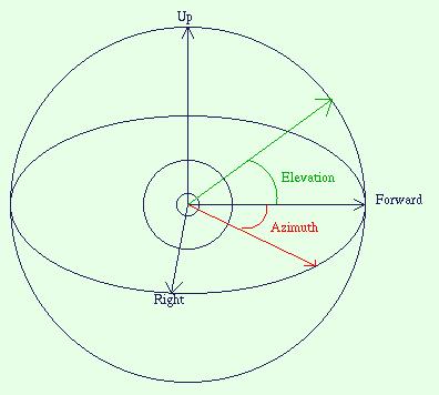
Coordinates for sound are given in spherical coordinates relative to the center of the head: (azimuth, elevation, distance) triples. Azimuth is measured in the horizontal plane with 0 degrees pointing straight forward. Elevation is measured in a vertical plane disecting the head perpendicular to the axis formed by the ears; again, 0 degrees is straight forward and intersects 0 degrees azimuth. Distance is simply the distance of the source.
The frequency composition of a signal can be extracted by means of the Fourier Transform. The Fourier Transform is defined as a function of an integral taken over the entire length of the signal wave. A signal is said to be in the time domain, and is graphed as amplitude versus time. The frequency content extracted by the Fourier Transform is measured in the frequency domain: amplitude versus frequency. The signal can be recomposed from its fourier transform via the inverse Fourier Transform which is almost identical: negating -i to i (square root of -1) produces the inverse Fourier Transform.
The Fourier Transform is linear, meaning that the Fourier Transform of signal A added to signal B is the sum of the Fourier transform of signal A with the Fourier Transform of signal B. Also multiplying the aplitude of a wave in the time domain also scales the Fourier Transform by the same factor.
Filters can be made by determining the how much each frequency should be scaled across the spectrum. Scalling a particular frequency by zero would perfectly reject it, while giving a value of two to another would double the signal intensity. This will be an amplitude vs. frequency graph, just as we would output from the Fourier Transform. We can then take the Fourier Transform of any signal and conduct a pairwise multiplication between the signals' frequencies and our scaling frequencies. We can then use the inverse Fourier Transform to return to the time domain where we will have a filtered signal. This can be simplified by use of the time domain equivalent of pointwise multiplication in the frequency domain: convolution. Convolution takes as input two waveforms in the time domain: the signal and the impulse response. It acts on these two waves and outputs a filtered wave. The impulse response is the inverse Fourier Transform of the frquency domain filter described above. If the filter we described were actually constructed, the impulse response would be the output of the filter when a signal containing all frequencies was input to it. A signal containing all frequencies is simply a spike of infinite amplitude and infintesimal duration, hence the name impulse response.