Schelling’s Model of Housing Segregation¶

Due: Friday, October 14th at 4pm

The goal of this assignment is to give you practice using nested loops, lists of lists, and functions.

You may work alone or in a pair on this assignment. The algorithms you need to implement for this assignment are more challenging than the first assignment. We recommend starting early.

Introduction¶

The New York Times has an interesting tool for viewing the distribution of racial and ethnic groups in cities and states around the country as recorded during the 2010 census. If you look at the map for the Greater Chicago area, you will see that many areas are heavily segregated, but that some, such as the suburb of Glendale Heights, are not. The forces that led to this arrangement of people are complex and it is unlikely that any simple model can truly answer the questions of how such segregation arises and why it persists. Keeping that in mind, one can still ask simple questions that may shed some light on the situation. In his 1978 book Micromotive and Macrobehavior, Thomas Schelling considered the following question: is it possible that a group of individuals would prefer to live in integrated neighborhoods and yet, as the result of their collective choices end up in segregated neighborhoods?

Schelling examined this question using a very simple model: A city has two kinds of people, Cubs fans and White Sox fans, for example, and each person in the city requires a certain number of his neighbors to be like him to feel comfortable in his location. Schelling used this model to study the patterns that emerge if, over time, people who are unsatisfied with their initial locations or become unsatisfied over time relocate to new locations that satisfy their criteria. What happens depends on the ratio of the two populations and on the satisfaction criteria used by the individuals, but segregation is a frequent outcome.

Your task in this assignment will be to implement a variant of Schelling’s model. Before you can do so, we need to specify the details of the model. In particular, we need to specify the:

shape and composition of a city,
boundaries of a home’s neighborhood,
definition for satisfaction,
rule for relocating unsatisfied homeowners,
composition of a step in the simulation, and
stopping conditions for the simulation.

Cities: A city is represented as an \(N \times N\) grid (where the value of \(N\) can be different for each city). Each grid location (or cell) represents a home, which can be in one of three states: open (that is, unoccupied), occupied by a red homeowner, or occupied by a blue homeowner. You can assume that a city has at least one open location.

In this assignment, you will always process the grid in row major order. That is, you will use a doubly-nested loop in which the index variable in the outer loop starts at zero and is used to indicate the current row, and the index variable in the inner loop starts at zero and is used to indicate the current column.

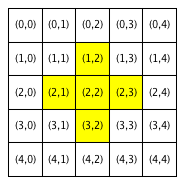
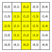
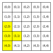
Neighborhood: The neighborhood of a home will be defined by a parameter R (this value will be an input to the model, so the value of R may vary from one simulation to another). The R-neighborhood of the home at Location \((i,j)\) contains all Locations \((k,l)\) such that \(0 \le |i-k| + |j-l| \le R\). Note that the Location \((i,j)\) itself is considered part of its own neighborhood. So, every homeowner will have at least one neighbor (himself).

We will refer to a neighborhood with parameter R=x as an “R-x neighborhood”. For example, the following figure shows the neighborhoods around Locations (2,2) and (3,0) when R=1 and when R=2. Cells colored yellow constitute the R-1 or R-2 neighborhood of Locations (2,2) and (3,0).

Neighborhood around (2,2)		Neighborhood around (3,0)
R = 1	R = 2	R = 1	R = 2

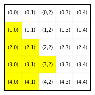Notice that Location (3,0), which is closer to the boundaries of the city, has fewer neighboring homes than Location (2,2), which is the middle of the city. We use the term boundary neighborhood to refer to a neighborhood that is near the boundary of the city and does not have a full set of neighbors.

Satisfaction: For each homeowner, we are going to compute a satisfaction score S + 0.5 * P where S is the number of neighbors of the same color and P is the number of open homes in the neighborhood. A homeowner is satisfied with his location, if the ratio of his satisfaction score to the number of homes in his neighborhood is greater than or equal to a specified threshold.

The two figures below show homeowners and their satisfaction status in a city with R-1 neighborhoods. The figure on the left was computed using a satisfaction threshold of 0.49, while the figure on the right was computed using a satisfaction threshold of 0.51. White locations are open. Blue (red) locations are occupied by satisfied blue (red) homeowners. Light blue (pink) locations are occupied by unsatisfied blue (red) homeowners.

Satisfaction threshold = 0.49	Satisfaction threshold = 0.51
R=1	R=1

The threshold is a parameter of the model, and will be the same for all the homeowners in a given simulation.

Relocation rule: If possible, an unsatisfied homeowner should be relocated to an open location that meets the satisfaction criteria. There may be more than one open home that would satisfy the homeowner. Our homeowners have little patience for house hunting, so they will take the first location they are offered that meets the criteria. They are also suspicious of homes that have been on the market too long, so they would prefer to look at locations with newly available homes first.

We will model the locations that are currently available with a list. To determine the new location for an unsatisfied homeowner, your implementation should try each open location on the list in order and relocate the homeowner to the first satisfactory location. If a satisfactory location is found, then it should be removed from the list and the homeowner’s previous home should be added to the front of the list of open homes. If none of the open locations are satisfactory, then the homeowner should not relocate.

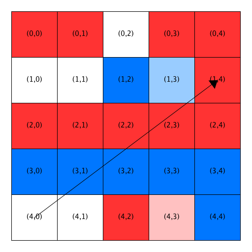
Here is an example relocation of the unsatisfied homeowner at Location (1,1) to Location (3, 3):

Before relocation	After relocation

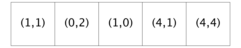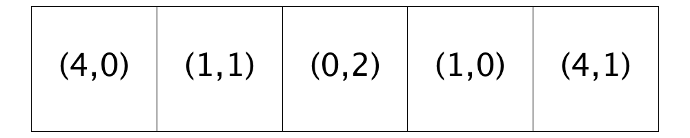
On the left, we show a city with R-1 neighborhoods with a satisfaction threshold of 0.51 along with a depiction of the locations that are open in the neighborhood (shown below the grid). The homeowner in Location (1,1) is unsatisfied with his location. Location (3,3) is the first location in the open location list that is satisfactory. The frame on the right shows the state of the neighborhood after this homeowner has been relocated. Notice that Location (3,3) has been removed from the list of open locations and Location (1,1) has been inserted into the front of the list. Also, notice that the homeowners in Locations (3,2) and (3,4) become satisfied when they gain a new blue neighbor at Location (3,3).

Simulation Step: During a simulation step, your code should attempt to relocate the homeowners who are unsatisfied at the start of the step to acceptable open locations. Your implementation will need to identify the unsatisfied homeowners and then try to relocate them one at a time. Please note that a homeowner will not relocate if he has become satisfied by the time he is processed.

To recap: a homeowner will relocate in a given step only if:

he was unsatisfied at the start of the step,
remains unsatisfied at the time at which he is processed, and
there is an open location that meets the satisfaction criteria.

Stopping conditions: Your simulation should stop when:

it has executed a specified maximum number of steps or
no relocations occur in a step.

Sample simulation: step 1

In the figure below, the first frame represents the initial state of a city. The next three frames illustrate the relocations that occur in the first step of the simulation.

Step 1
Initial state	After 1st relocation	After 2nd relocation	After 3rd relocation

At the start of step 1, there are unsatisfied homeowners at locations (1,1), (1, 4), (2, 4), (3, 0), (3, 2), (3, 4), and (4, 0). Here is what happens as we process each homeowner in this list:

The first two open locations are not satisfactory for the blue homeowner at (1,1), so he is relocated to Location (3,3). Notice that Location (3,3) has been removed from the list of open locations and Location (1,1) has been added to the front of the list. Also notice that the homeowners in Locations (3,2) and (3,4) become satisfied when a blue person relocates into the previously open home between them.
The homeowner at Location (1, 4) relocates to Location (4,4). Notice that this change causes the homeowner in Location (2, 4) to become satisfied with his location, while the homeowner in Location (1, 3) becomes unsatisfied when he loses a blue neighbor and the homeowner in Location (4, 3) becomes unsatisfied when he gains a blue neighbor in the previously empty home next to him.
The homeowner in (2, 4) is now satisfied, so he does not relocate.
The homeowner in (3, 0) remains unsatisfied. There is no suitable open location available, so he does not relocate.
The homeowners in (3, 2) and (3,4) are now satisfied, so they do not relocate.
The homeowner in Location (4, 0) relocates to Location (1, 4). In the process, the homeowner at Location (3, 0) becomes satisfied.

Notice that the two homeowners who became unsatisfied during the step were not relocated during the step.

Sample simulation: step 2

The first frame in the figure below represents the state of a city at the start of the second step. Notice that both the state of the grid and the open locations list are the same as they were at the end of the first step.

Step 2
Initial state	After 1st relocation	After 2nd relocation

There are two unsatisfied homeowners, at Locations (1, 3), and (4, 3), at the start of the step. During the step, these homeowners are relocated to Locations (4, 0) and (1, 3) respectively. Two homeowners, at Location (1,2) and (4, 2), become unsatisfied during the step.

Sample simulation: step 3

The first frame in the figure below represents the state of a city at the start of the third step.

Step 3
Initial state	After 1st relocation	After 2nd relocation

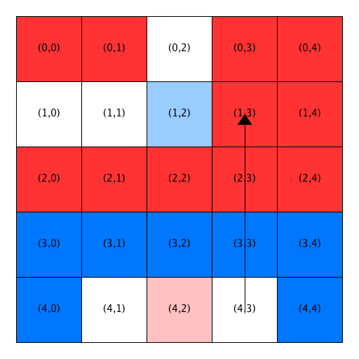
During this step, the homeowner at Location (1, 2) is relocated to the recently vacated Location (4, 3) and, in turn, the homeowner at Location (4, 2) is relocated to Location (1,2).

Sample simulation: step 4

The first frame in the figure below represents the state of a city at the start of the fourth step. At this point, all the homeowners are satisfied, so no relocations are done during the fourth and the simulation halts.

Step 4
Initial state	Final state

Notice how, in our model, homeowners can be satisfied even if some of their neighbors are different from them and, yet, the relocations result in a completely segregated city.

Data representation¶

Your implementation will need a representation for the current state of a homeowner, a representation for the city (aka the grid), a representation for the locations that are currently open (unoccupied), and a representation for the list of locations with homeowners who are unsatisfied at the start of a step.

Representing Homeowners/Homes: Homeowners will be represented by the strings “B” and “R”, and open homes are represented by “O”.

Representing cities: We will represent a city using a list of lists with strings as elements. You can assume that these strings will always be one of “B”, “R”, or “O”.

The directory pa2/tests contains text representations of some sample city grids, including all of the grids shown above (see tests/sample-grid.txt). See the file tests/README.txt for descriptions of the grid file format and the grid files included in the tests sub-directory.

The file utility.py contains some useful functions for working with grids:

is_grid(grid): does grid have the right type and shape to be a city grid?
read_grid: takes the name of a grid file as a string and returns a grid. sample use: utility.read_grid("tests/sample-grid.txt") (assumes utility has been imported).
print_grid(grid): takes a grid and prints it to stdout.
find_mismatch(grid0, grid1): takes two grids and returns the first location at which they differ. This function returns None if the grids are the same.

Representing Locations: We will use pairs (tuples) of integers to represent locations.

Tracking open locations We will use a list of pairs (locations) for tracking open locations.

Your implementation should initialize the list of open locations from the grid at the start of a simulation. It will be updated whenever a homeowner relocates.

When looking for a new location for a homeowner, your implementation will walk through the list of open locations in order starting at index 0 and use the first location that is satisfactory, if such a location exists. If you find that Location (i, j) at index \(x\) in the open locations list is appropriate for the homeowner currently at Location (k, l), you should remove the location at index \(x\) from the list (using del or pop) and add Location (k, l) to the beginning of the list (using insert).

We encourage you to look carefully at the open locations list in the example above. In particular, notice that we do not recompute the list of open locations between steps.

Representing Unsatisfied Homeowners We will use a list of location pairs, which will be recomputed at the start of every step, for representing the unsatisfied homeowners

Code structure¶

Your task is to implement a function:

def do_simulation(grid, R, threshold, max_num_steps)

that executes simulation steps on the specified grid until one of the stopping conditions is met. This function must return the number of steps executed. Your function can and should modify the grid argument. At the end of the simulation, the grid should reflect the relocations that took place during the simulation.

When designing your function decomposition, keep in mind that you need to do the following subtasks:

identify whether a homeowner is satisfied at a particular location;
create and initialize the list of open locations;
create and initialize the list of unsatisfied homeowners;
attempt to relocate an owner to a new location;
simulate one step of the simulation;
run steps until one of the stopping conditions is met.

We kept Tasks 4 and 5 separate, but you may find it easier to combine them into one task. Do not combine the last three tasks into one mega-task, because the resulting code would be hard to read and debug.

Testing¶

We have provided some test code for you, but you will also need to write some test code of your own.

Testing satisfaction

To encourage you to separate out the task of determining whether a homeowner is satisfied at a particular location, we have provided test code for such a function. Our code assumes that you have written a function with the header:

def is_satisfied(grid, R, threshold, location)

for determining whether the homeowner at the specified location is satisfied given the specified grid, value for R, and threshold.

For each test case, our test code reads the input grid from a file, calls your is_satisfied function with the grid and the other parameters specified for the test case, and checks the actual result against the expected result. Here is a description of the tests and their purpose:

Tests for `is_satified`¶
Test number	Grid filename	R	Location	Threshold	Expected result	Purpose
0	sample-grid.txt	1	(0, 0)	0.823333	True	Check boundary neighborhood:top left corner.
1	sample-grid.txt	1	(0, 0)	0.843333	False	Check boundary neighborhood:top left corner.
2	sample-grid.txt	2	(0, 0)	0.656667	True	Check boundary neighborhood: top left corner.
3	sample-grid.txt	2	(0, 0)	0.676667	False	Check boundary neighborhood: top left corner.
4	sample-grid.txt	1	(0, 4)	0.656667	True	Check boundary neighborhood: top right corner.
5	sample-grid.txt	1	(0, 4)	0.676667	False	Check boundary neighborhood: top right corner.
6	sample-grid.txt	2	(0, 4)	0.573333	True	Check boundary neighborhood: top right corner.
7	sample-grid.txt	2	(0, 4)	0.593333	False	Check boundary neighborhood: top right corner.
8	sample-grid.txt	1	(4, 0)	0.490000	True	Check boundary neighborhood: lower left corner.
9	sample-grid.txt	1	(4, 0)	0.510000	False	Check boundary neighborhood: lower left corner.
10	sample-grid.txt	2	(4, 0)	0.573333	True	Check boundary neighborhood: lower left corner.
11	sample-grid.txt	2	(4, 0)	0.593333	False	Check boundary neighborhood: lower left corner.
12	sample-grid.txt	1	(1, 1)	0.490000	True	Check neighborhood that is complete when R is 1.
13	sample-grid.txt	1	(1, 1)	0.510000	False	Check neighborhood that is complete when R is 1.
14	sample-grid.txt	2	(1, 1)	0.444545	True	Check neighborhood that is not complete when R is 2.
15	sample-grid.txt	2	(1, 1)	0.464545	False	Check neighborhood that is not complete when R is 2.
16	grid-no-neighbors.txt	1	(2, 2)	0.590000	True	Check interior neighborhood with location that has no neighbors.
17	grid-no-neighbors.txt	1	(2, 2)	0.610000	False	Check interior neighborhood with location that has no neighbors.
18	grid-no-neighbors.txt	2	(2, 2)	0.643846	True	Check interior neighborhood with a location that has no neighbors.
19	grid-no-neighbors.txt	2	(2, 2)	0.663846	False	Check interior neighborhood with a location that has no neighbors.
20	grid-no-neighbors.txt	1	(4, 4)	0.656667	True	Check boundary neighborhood (lower right corner) with location that has no neighbors.
21	grid-no-neighbors.txt	1	(4, 4)	0.676667	False	Check boundary neighborhood (lower right corner) with location that has no neighbors.
22	grid-no-neighbors.txt	2	(4, 4)	0.406667	True	Check boundary neighborhood (lower right corner) with location that has a few neighbors.
23	grid-no-neighbors.txt	2	(4, 4)	0.426667	False	Check boundary neighborhood (lower right corner) with location that has a few neighbors.
24	grid-lone-blue-sea-of-red.txt	1	(3, 3)	0.190000	True	Check one blue homeowner in an all red neighborhood.
25	grid-lone-blue-sea-of-red.txt	1	(3, 3)	0.210000	False	Check one blue homeowner in an all red neighborhood.
26	grid-lone-blue-sea-of-red.txt	2	(3, 3)	0.080909	True	Check one blue homeowner in an all red boundary neighborhood.
27	grid-lone-blue-sea-of-red.txt	2	(3, 3)	0.100909	False	Check one blue homeowner in an all red boundary neighborhood.
28	sample-grid.txt	3	(2, 2)	0.513810	True	R is 3.
29	sample-grid.txt	3	(2, 2)	0.533810	False	R is 3.

All of the grid files can be found in the tests subdirectory.

There are many corner cases for this function, but that does not mean that your code needs to be complex!

As in PA #1, we will be using py.test to test your code. You can run these tests with the command:

py.test -xv test_is_satisfied.py

Recall that the -x flag indicates that pytest should stop when a test fails. The -v flag indicates that pytest should run in verbose mode. And the -k flag allows you to reduce the set of tests that is run. For example, using -k test_0 will only run the first test.

Testing the full simulation

We have also provided test code for do_simulation. For each test case, our code reads in the input grid from a file, calls your do_simulation function, checks the actual state of the grid against the expected state of the grid, and checks the actual number of steps returned by do_simulation with the expected number of steps.

Here is a description of the tests and their purpose:

Tests for `test_do_simulation`¶
Test number	Input grid filename	Expected grid filename	R	Threshold	Maximum number of steps	Expected numer of steps	Purpose
0	tests/sample-grid.txt	tests/sample-grid-1-51-0-final.txt	1	0.51	0	0	Check stopping condition #1
1	tests/sample-grid.txt	tests/sample-grid-1-49-2-final.txt	1	0.49	2	1	All homeowners statisfied at the start. Check stopping condition #2
2	tests/sample-grid.txt	tests/sample-grid-1-51-1-final.txt	1	0.51	1	1	Check sample grid after 1 simulation step
3	tests/sample-grid.txt	tests/sample-grid-1-51-2-final.txt	1	0.51	2	2	Check sample grid after 2 simulation steps
4	tests/sample-grid.txt	tests/sample-grid-1-51-3-final.txt	1	0.51	3	3	Check sample grid after 3 simulation steps
5	tests/sample-grid.txt	tests/sample-grid-1-51-4-final.txt	1	0.51	4	4	Check sample grid after 4 simulations steps
6	tests/sample-grid.txt	tests/sample-grid-1-51-5-final.txt	1	0.51	5	4	Check stopping condition #2
7	tests/grid-lone-blue-sea-of-red-2.txt	tests/grid-lone-blue-sea-of-red-2-1-40-2-final.txt	1	0.40	2	1	Check case where possible new location is in the homeowner’s current neighborhood
8	tests/sample-grid.txt	tests/sample-grid-2-51-7-final.txt	2	0.51	7	7	Check sample grid with R of 2
9	tests/sample-grid.txt	tests/sample-grid-2-51-8-final.txt	2	0.51	8	7	Check stopping condition #2
10	tests/sample-grid.txt	tests/sample-grid-3-51-5-final.txt	3	0.51	5	5	Check sample grid with R of 3
11	tests/grid-150-40-40.txt	tests/grid-150-40-40-3-51-100-final.txt	3	0.51	100	41	Check efficiency using large grid with R of 3

All of the grid files can be found in the tests subdirectory.

You can run:

py.test -xv -k "not large" test_do_simulation.py

to run all the tests except the one that uses the large grid.

We strongly encourage you to test your intermediate functions. You do not need to do anything fancy. For example, you could fire up ipython3, load your code, use our function to read a grid from a file, and run the code that simulates a single relocation (or a single step, which might have multiple relocations), and then either inspect the result or read the expected grid from a file and test whether your actual grid matches the expected grid. You could even put this set of steps in a simple function and use it multiple times! The surest way to guarantee that you will need to spend hours debugging your code is to start your testing at do_simulation.

Running your program¶

The main function supplied in schelling.py parses the command-line arguments, reads a grid from a file, calls your do_simulation function, and then prints the resulting grid.

The command line arguments are: the name of the input grid file, a value for R, a value for the satisfaction threshold, and a maximum number of steps. For example, running the following command:

python3 schelling.py tests/sample-grid.txt 1 0.51 1

will do a simulation using the grid specified in the file tests/sample-grid.txt, with R=1, a threshold of 0.51, and a maximum number of steps of 1.

Drawing a grid¶

We have provided some code to allow you to look at a pictorial representation of a grid similar to those shown in the assignment description. The figures show whether a home is empty, occupied by a red homeowner, or occupied by a blue homeowner. They do not include any indication of whether the homeowner is satisfied. To use this code, run the following command in a Linux terminal window:

./drawgrid.sh <grid filename>

where <grid filename> is replaced with the name of a grid file. For example, to draw the grid in tests/sample-grid.txt, you would run the command:

./drawgrid.sh tests/sample-grid.txt

This program will pop up a new window with the drawing. To exit, click on the red circle on the top-left part of the window.

Grading¶

Writing code that produces the correct answer is not sufficient. You must also write clean and well organized code. Specifically, your submission will be graded on:

Correctness on our do_simulation tests (~20%)
Function decomposition, code structure, and style (~25%)
Implementation details (~55%)

Getting started/Submission¶

See these start-up and submission instructions if you intend to work alone.

See these start-up and submission instructions if you intend to work in a pair.

Acknowledgments: This assignment was inspired by a discussion of Schelling’s Model of Segregation in Housing in the book Networks, Crowds, and Markets by Easley and Kleinberg. The definition of a neighborhood and the method for choosing a new location for an unsatisfied homeowner were inspired by the paper The (In)compatibility of Diversity and Sense of Community by Z. Neal and J. Waiting Neal.