Visualizing Time Use Data Using TreeMaps

Due: Wednesday, Nov 30th at 4pm.

Please note the non-standard due date.

The purpose of this assignment is to give you practice working with recursive data structures and writing recursive functions.

You must work alone on this assignment.

Introduction

The Bureau of Labor Statistics (BLS), which is a division of the U.S. Department of Labor, is the principal Federal agency responsible for measuring labor market activity, working conditions, and price changes in the economy. Its mission is to collect, analyze, and disseminate economic information to support public and private decision-making.

BLS gathers an incredible array of data. In this assignment, we will be working with data from the American Time Use Survey (ATUS). You can learn about the detailed history of this survey and about how the results can be used in the American Time Use Survey User’s Guide. For our purposes, it is sufficient to see the Guide’s description of what the survey measures and how it is gathered:

The American Time Use Survey (ATUS) is the Nation’s first federally administered, continuous survey on time use in the United States. The goal of the survey is to measure how people divide their time among life’s activities.

In ATUS, individuals are randomly selected from a subset of households that have completed their eighth and final month of interviews for the Current Population Survey (CPS). ATUS respondents are interviewed only one time about how they spent their time on the previous day, where they were, and whom they were with. The survey is sponsored by the Bureau of Labor Statistics and is conducted by the U.S. Census Bureau.

The major purpose of ATUS is to develop nationally representative estimates of how people spend their time. Many ATUS users are interested in the amount of time Americans spend doing unpaid, non-market work, which could include unpaid childcare, eldercare, housework, and volunteering. The survey also provides information on the amount of time people spend in many other activities, such as religious activities, socializing, exercising, and relaxing. In addition to collecting data about what people did on the day before the interview, ATUS collects information about where and with whom each activity occurred, and whether the activities were done for one’s job or business. Demographic information—including sex, race, age, educational attainment, occupation, income, marital status, and the presence of children in the household—also is available for each respondent. Although some of these variables are updated during the ATUS interview, most of this information comes from earlier CPS interviews, as the ATUS sample is drawn from a subset of households that have completed month 8 of the CPS.

The data collected from each ATUS participant is quite detailed. The full data set includes a code that identifies a specific participant, the time an activity started, the time it ended, the type of activity, and who else was with the participant when the activity occurred, for every activity engaged in by each participant during a 24 hour period. We will be using the summary form of the data which includes the total amount of time spent by the participant on each type of activity.

The summary data can be represented hierarchically. For example, below we show an abridged version of one participant’s summary data. Each line includes a numeric code for the category of activity, known as the time use code, the name of the category, and the amount of time (in minutes) the participant spent on activities from that category. We use nesting to show the hierarchy.

01: Personal Care 600
    0101: Sleeping 565
        010101: Sleeping 565
    0102: Grooming 35
        010201: Washing, dressing and grooming oneself 35
02: Household Activities 316
    0201: Housework 120
        020101: Interior cleaning 120
    0202: Food & Drink Prep., Presentation, & Clean-up 115
        020201: Food and drink preparation 55
        020203: Kitchen and food clean-up 60
    0205: Lawn, Garden, and Houseplants 20
        020501: Lawn, garden, and houseplant care 20
    0206: Animals and Pets 41
        020601: Care for animals and pets (not veterinary care) 1
        020602: Walking / exercising / playing with animals 40
    0209: Household Management 20
        020904: HH & personal e-mail and messages 20
11: Eating and Drinking 50
    1101: Eating and Drinking 50
        110101: Eating and drinking 50
12: Socializing, Relaxing, and Leisure 474
    1201: Socializing and Communicating 20
        120101: Socializing and communicating with others 20
    1203: Relaxing and Leisure 454
        120303: Television and movies (not religious) 360
        120305: Listening to the radio 30
        120312: Reading for personal interest 64

This participant reported zero minutes for the more than 400 categories that are not shown. While this data is vaguely interesting in this form, it takes some careful study to get a sense how this person spends his time. It would be much better to see a visual representation of the data.

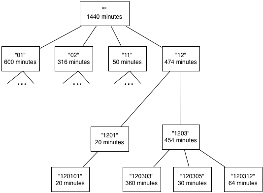
One way to visualize this data, as a tree of the form we have seen in class, directly reflects the hierarchical nature of the data:

Sample participant data formatted as a tree.

Note that we have used the time use codes rather than the category names to identify the nodes and elided the descendants of 01, 02, and 11 for the sake of compactness. Also, we added a root node (time code: “”, minutes:1440) to tie the categories together into a single tree.

This visualization still does not give us an intuitive sense of the relative amount of time spent on different activities. For example, 360 minutes were spent on 120303 but, to get some context on how large or small that amount is, we need to look at its parent nodes. So, 360 minutes is a “large” amount in the context of its immediate parent (1203, which has a total of 454 minutes), but not so large in the context of the entire tree (which has a total of 1440 minutes).

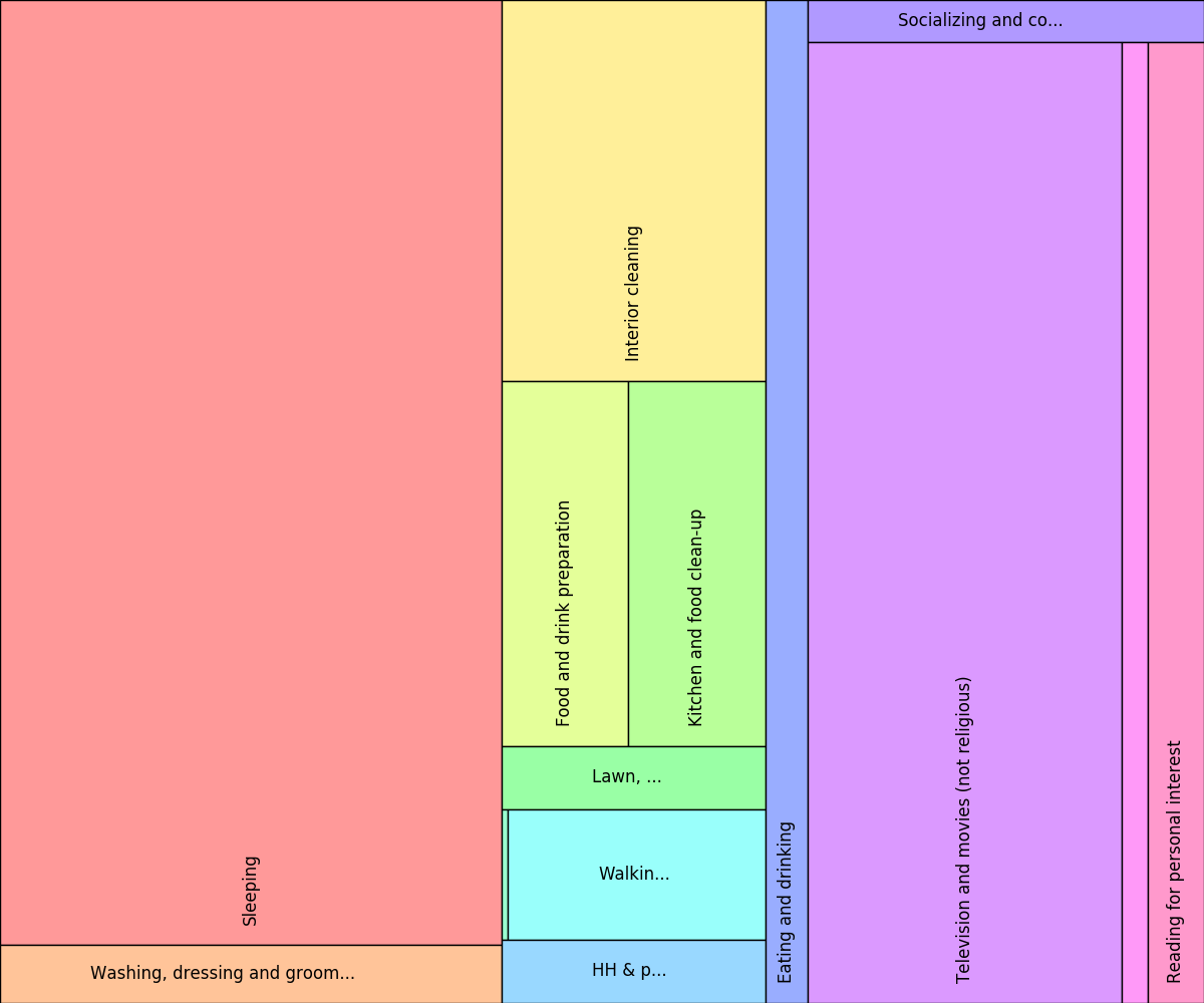
How can we visualize this information in an effective way? We can use Treemaps, which are an excellent tool for visualizing hierarchical data. Here, for example, is a treemap for our sample participant:

Treemap for sample participant

Looking at the data in this form, it is immediately clear that this participant spends way more time watching TV and movies than he does socializing with friends.

More generally, treemaps are a space-constrained method for visualizing hierarchical structures that present a sense of “mass” and proportionality in a way that the typical tree diagram shown above does not. Treemaps allow users to compare leaves and sub-trees even at varying depths in the tree, and spot patterns and exceptions. Ben Shneiderman designed treemaps during the 1990s as a way to visualize the contents of a file system. This technique has since been used to visualize many different types of data including stock portfolios, oil production, a gene ontology, stimulus spending, and more. The original idea has been extended in lots of interesting ways.

In this assignment, you will write code to draw treemaps. Before we explain how to draw a treemap, we will describe the ATUS data in more detail.

American Time Use Survey

Structure of the Time Use Categories

The time use categories are assigned codes that form a three tier hierarchy. The first tier uses a two digit code to represent 17 different major activity categories, such as, Personal Care (01) or Household Activities (02). The second tier uses four digit code, the first two of which specify a Tier 1 category, and the second two of which describe a specific subcategory of that Tier 1 category. For example, the sub-categories of Personal Care (01) are:

0101: Sleeping
0102: Grooming
0103: Health-related Self Care
0104: Personal Activities
0105: Personal Care Emergencies
0199: Care, n.e.c.

where “n.e.c.” stands for Not elsewhere classified. Finally, the Tier 3, or the most detailed, categories are represented by a six digit code that comprises a four digit Tier 2 category followed by a two digit code for a specific activity within that Tier 2 category. For example, the sub-categories of Grooming (0102) are:

010201: Washing, dressing and grooming oneself
010299: Grooming, n.e.c.

The structure of the ATUS data is not necessarily consistent across years. We will be using data from the 2015 survey.

Participant summary data

The summary data is stored in a CSV file. The first row is a header that describes the contents of each column. The columns with labels that start with a “t” and are followed by a six digit time use code contain information about minutes spent in the associated time use category.

There is one row in this file for every participant in the sample. We can use the tier structure of the time use codes to build a tree like the one shown above for the summary data of a specific participant. In our figures, each node in the tree has a time use code, a number of minutes, and zero or more children. Our representation for the tree nodes also includes a field that we can use to store the name of the time use category.

Representing tree nodes

We provide a class, TreeNode, that you can use to represent tree data. The class is useful for representing ATUS summary data, but it is not specific to the ATUS data.

Take into account that this is not the same Tree class we saw in class. However, its internal representation is very similar: a TreeNode object represents a node on a tree, each node has a series of attributes, and the node’s children are stored in a dictionary (instead of a list). The public interface for this class includes:

• a constructor for creating a tree node,
• properties for a code attribute (string), a label attribute (string), and a weight attribute (float),
• a setter for the weight,
• a method, get_children_as_list, for accessing the node’s children, and
• for debugging purposes, a method for printing the tree rooted at the node (print_tree).

We can use this class to represent our ATUS data by using the code attributes to hold the time use code, the label attribute to hold the time use category name, and the weight attribute to hold the number of minutes spent a particular category. We set the code and label for the root node to the empty string and the weight for all interior nodes to zero when the tree is constructed.

If you are wondering why we are using generic names—code, label and weight— rather than time use code, time use category and minutes, it is because this approach allows your treemap implementation to be more generically useful. You’ll see a tree map for a different data set later in the assignment.

Drawing Treemaps

The treemap algorithm takes a weighted tree—where the weight of a leaf is an application-specific cost and the weight of a subtree is the sum of the weights of its children—and an initial bounding rectangle as arguments. It assigns regions in the rectangle to the leaves of the tree. The size of the region assigned to a leaf (itself a rectangle) is a function of the leaf’s relative weight and its placement is a function of its position in the tree.

Here is an example that we will use to make this concept more concrete:

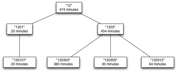
Sample participant: Time code 12 tree

This tree represents the socializing, relaxing, and leisure activities (code 12) for the sample participant discussed above.

To explain how the treemap algorithm works, we need to describe how to:

1. compute the weights,
2. represent rectangles,
3. partition the initial bounding rectangle,
4. use the drawing package, and finally
5. choose the colors and labels for the rectangles in the resulting partition.

Weighting Function:

The weights of the leaves are set at the time the tree is constructed and can be accessed using the weight property. The weight of the interior nodes needs to be computed and for a given interior node should be set to the sum of the weights of its children. In our example, the nodes labelled 120303, 120305, and 120312 have weights 360, 30 and 64 respectively and so, the weight of their parent node (1203) is set to 454. Similarly, the weight of the 12 node is 474, which is the sum of the weights of its children (20 and 454).

Representing rectangles

A rectangle can be represented using points on two opposing corners (upper left and lower right corners, for example) or a single point (the origin) and a width and a height. We use the latter representation for our implementation and in this description, but either works. In most of our examples below, we use a bounding rectangle that has an origin of (0, 0), a height of 1.0, and a width of 1.0. (Note: these values are naturally unit-less.)

It will be helpful when you try to interpret the diagrams below to know that the origin (0,0) for our coordinate system is in the upper left corner, rather than lower left corner, which might seem more natural. We made this choice, because this coordinate system matches the coordinate system of many drawing packages, including ours.

Partitioning the initial bounding rectangle

Once the tree is decorated with the correct weights, we need to divide an initial bounding rectangle into a collection of smaller rectangles based on the shape of the tree and the distribution of the weights (“mass”). Each rectangle in the resulting partition will have an associated code and label.

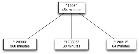
To describe how regions of the bounding rectangle are allocated in the treemap algorithm, we will start by looking at the treemap for the 1203 subtree from our example above.

Sample participant: Time code 1203 - tree & treemap

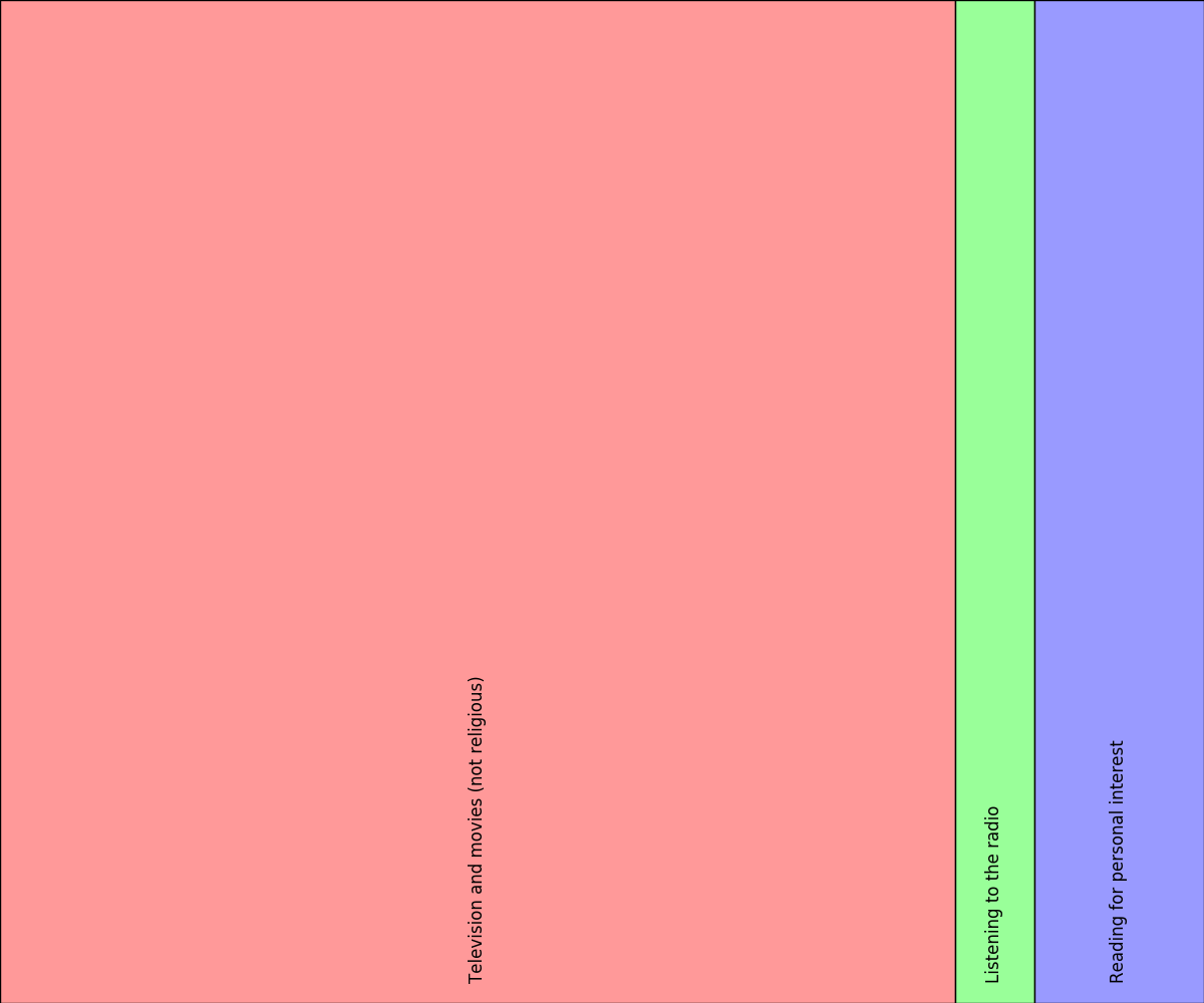The treemap algorithm splits the initial rectangle into sub-rectangles—one per child of the root. The proportion of a child’s sub-rectangle is determined by its weight as a fraction of the total weight of its parent. For example, the treemap algorithm splits the initial rectangle assigned to the 1203 node into three pieces from left to right. Given an initial bounding rectangle with its origin at (0,0), a width of 1.0 and a height of 1.0, the resulting partition would be:

Sample participant: Time code 1203 - partition

Code	X	Y	Width	Height	Label
120303	0.000	0.000	0.793	1.000	120303: Television and movies (not religious)
120305	0.793	0.000	0.066	1.000	120305: Listening to the radio
120312	0.859	0.000	0.141	1.000	120312: Reading for personal interest

Each row corresponds to a rectangle and each rectangle is associated with a node in the tree. In this case, the rectangles are associated with the leaves of the 1203 subtree. The first column identifies the tree nodes’ time use codes, the next four contain the components of the rectangles (rounded to three digits for clarity), and the final column contains the nodes’ labels. Notice that 79.3% of the initial rectangle (by width) went to 120303, 6.6% went to 120305, and 14.1% 120312, which corresponds to their relative weights of 360/454, 30/454, 64/454.

Moving on to the 12 subtree:

Sample participant: Time code 12 - tree and treemap

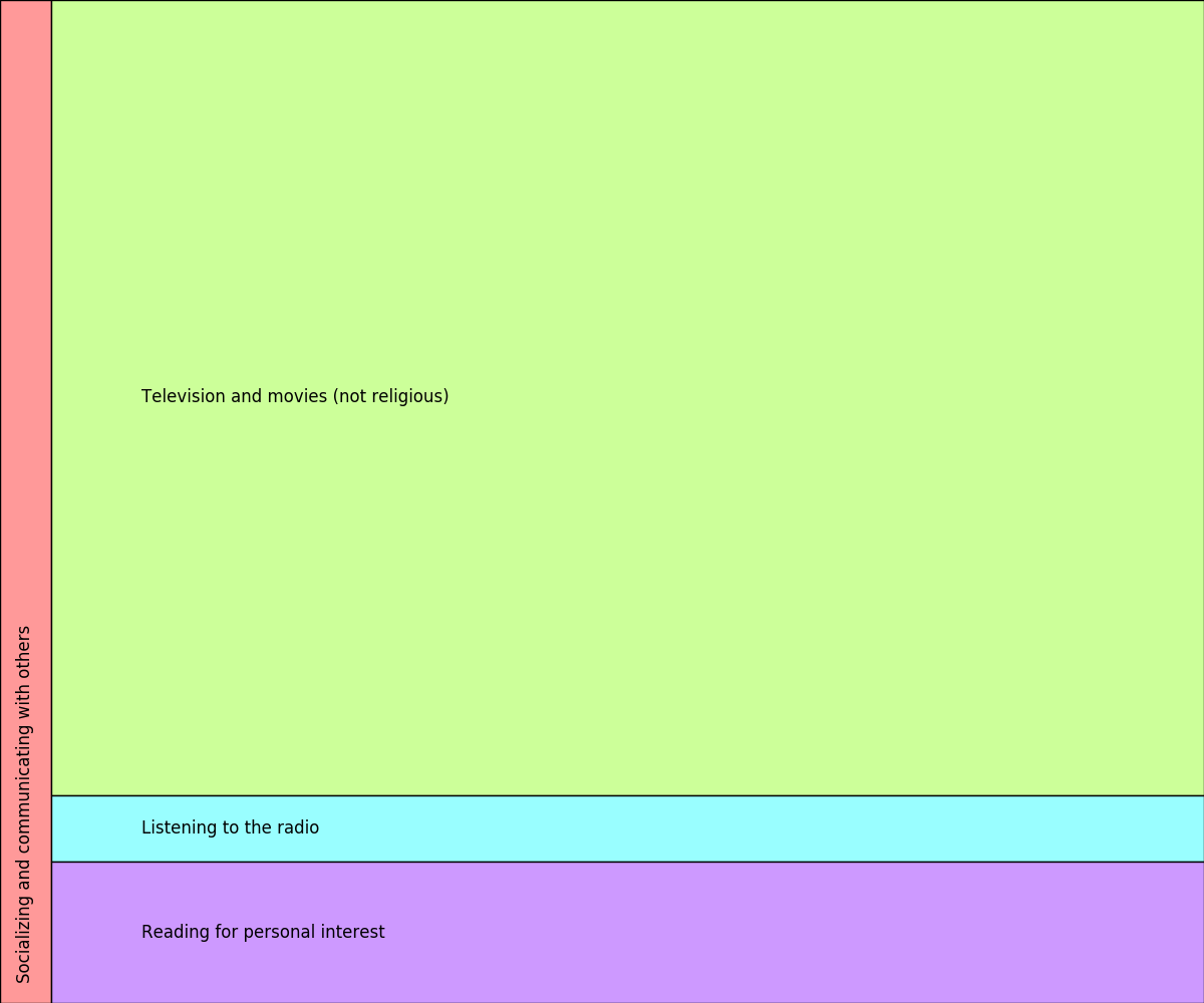The treemap algorithm splits the initial rectangle assigned to the 12 node from left to right into two rectangles with 4.2% of the width of the initial rectangle going to the 1201 subtree and the remaining 95.8% going to the 1203 subtree. The 1203 rectangle is further subdivided as described earlier. Notice that while the proportions of the 1203 split are the same as the earlier picture, the split dimension and the orientation of the corresponding rectangles has changed. If the initial bounding rectangle had its origin at (0,0), a width 1.0, and a height 1.0, the resulting partition would be:

Sample partiticpant: Time code 12 - partition

Code	X	Y	Width	Height	Label
120101	0.000	0.000	0.042	1.000	120101: Socializing and communicating with others
120303	0.042	0.000	0.958	0.793	120303: Television and movies (not religious)
120305	0.042	0.793	0.958	0.066	120305: Listening to the radio
120312	0.042	0.859	0.958	0.141	120312: Reading for personal interest

The orientation of the partitions alternates as we move down the tree. The rectangle assigned to the 12 node was split left-to-right. The rectangles assigned to the Tier 2 nodes (1201 and 1203) were split top-down when necessary. Alternating the split at each level in the tree produces a picture that is much easier to understand than one in which all the partitions have the same orientation.

Finally, here is the treemap for whole tree for the sample participant:

Treemap for sample participant

The orientation of the partitions again alternates. The rectangle assigned to the root of the tree was split left-to-right. The Tier 1 rectangles were split top-down, and finally, the Tier 2 rectangles were split left-to-right.

During the course of running the treemap algorithm, you may generate a rectangle that is too small to be useful. In this case, do not split it any further. We will define a rectangle to be too small to split further if it has a height or a width less than 0.01. (We have defined a constant, MIN_RECT_SIDE, in treemap.py, for this purpose.)

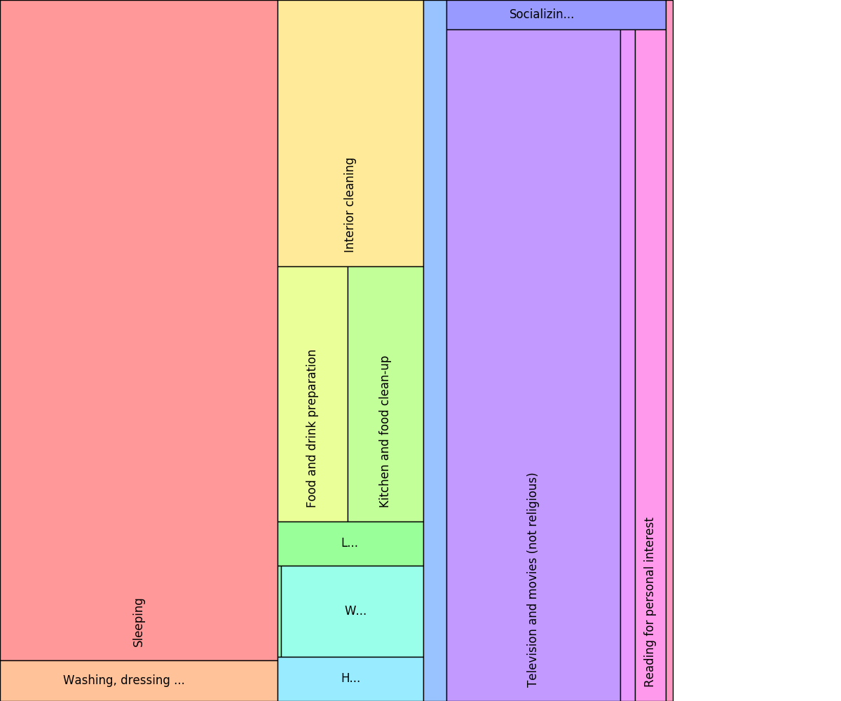
To illustrate this behavior, we constructed a synthetic participant by cloning our sample participant and adding three five minute activities to the Traveling category (18). If we construct a treemap with an initial rectangle with an origin at (0,0), a non-standard starting width of 0.8, and a height of 1.0, we get we get the following figure:

Treemap for a synthetic participant with initial width of 0.8

The very slim rectangle at the right edge of the treemap represents the activities that fall under time code 18. This rectangle was too small to split further. (Please note that when you draw this example, you’ll see a white strip of width 0.2 on the right-hand side, because the treemap is not using the full-width of the underlying canvas.)

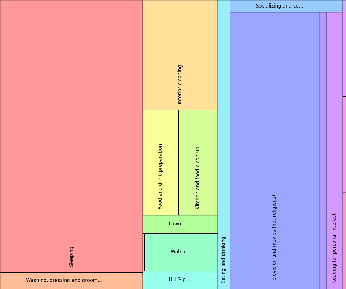
If you draw the same figure with the standard initial rectangle (1.0 instead of 0.8), the rectangle assigned to the node for time code 18 is larger and gets split into three parts:

Treemap for synthetic participant with initial with of 1.0

Using the drawing package

We will be using the ChiCanvas class for drawing rectangles and text. This class provides a way to create a canvas, draw the outline of a rectangle, draw a rectangle filled with a particular color, draw text horizontally and vertically, show a drawing, etc. See the API for details. The file sample.py contains a set of simple examples that use this class.

Our code handles the construction of a canvas for you. The coordinate system for the canvas is the unit square with an origin of (0.0, 0.0) (upper left corner), a width of 1.0, and a height of 1.0. Again, these values are unit-less.

We strongly encourage you to look carefully at the ChiCanvas API and at sample.py before you get started with drawing.

The ColorKey class allows you to create a key that maps codes to colors (API). The constructor takes a set of codes as strings and assigns colors to the code. Given a ColorKey named ck, you extract the color for a particular code, c, with the get_color_method. For example:

ck.get_color(c)

This class also has a method for drawing a key that shows the mapping of colors to code, but we will not use it for this assignment.

Choosing labels and colors

Each rectangle in the partition that results from the previous step is associated with a tree node.

It may appear that you will get one color per leaf, but this assumption is incorrect. An interior node might have a very small weight relative to the rest of the tree and as a result, the partitioning algorithm will not split its assigned rectangle any further. Also, while the codes associated with the tree nodes are unique in the ATUS data set, you may not assume that is true for all data sets. [Hint: we found the Python set data structure useful when compiling the codes for the color key.]

You will construct a color key using the codes from the nodes in your partition and then use this key and the codes to determine the appropriate colors when you draw the partition rectangles. For example, your color key for the treemap for 1203 subtree would have three colors, one each for 120303, 120305, and 120312.

You should orient the labels in the rectangles horizontally or vertically depending on whether the width or the height of the rectangle is larger. If the width and the height are the same, orient the labels horizontally. Do not draw the label for any rectangle that has a height or width of less than .03. (We have defined a constant, MIN_RECT_SIDE_FOR_TEXT for this purpose.) Note that labels that are too long will be clipped to fit automatically by the drawing package.

Your task

Your task is to complete the function:

def draw_treemap(t,
                 bounding_rec_height=1.0,
                 bounding_rec_width=1.0,
                 output_filename=None)

in treemap.py, which takes a tree, the height and width of initial bounding rectangle, and an optional filename, and constructs a canvas and then draws a tree map for t using the specified initial rectangle. If the output filename is None, then your code should “show” the canvas. Otherwise, it should save the canvas in the specified file.

Your functions for computing the weights and the partition must be recursive. Also, you may not make any assumptions about the number of levels in the tree.

You are on your own for deciding what functions to write. We highly recommend that you figure out what functions you need before you start writing code and test those functions as you go. Our solution has four functions, including draw_treemap, and is roughly 50 lines of code.

Testing

We have provided a function, load_participant, to simplify testing. This function takes a participant’s line number in the participant file and an optional time code and constructs a tree for that participant and returns it. If a time code is supplied, it is used as a path to a subtree and the subtree is returned.

To do small scale testing fire up ipython3, and then run atus.py to load the code, load a tree or subtree using load_participant and then call the function(s) you want to test. You can use the print_tree method to examine the state of the tree.

The follow example loads the “1203” subtree for participant #1 and then prints the tree.

In [2]: t = load_participant(1, time_code="1203")

In [3]: t.print_tree()
1203 Relaxing and Leisure 0
    120303 Television and movies (not religious) 360
    120305 Listening to the radio 30
    120312 Reading for personal interest 64

For more large scale testing, you can recreate the sample treemaps shown above by running atus.py with the appropriate arguments (see tab-commands).

Commands for generating the example treemaps

fig-sp-treemap	python3 atus.py -p 1
tab-time-code-1203 (right)	python3 atus.py -p 1 -c 1203
tab-time-code-12 (right)	python3 atus.py -p 1 -c 12
fig-syn-treemap-narrow	python3 atus.py -p 2 -w 0.8
fig-syn-treemap	python3 atus.py -p 2

Second data set

Up to this point, we have only discussed trees built from ATUS summary data. The algorithm as described only requires that the data you want to visualize is represented as a tree and that you have access to certain kinds of information using specific property and function names. As long as the class of the tree parameter (t) has properties for code, label, and weight, a setter for weight, and an appropriate function named get_children_as_list, you should be able to draw a treemap for t using your implementation.

The code in the file fdic.py builds a tree using data from the Federal Deposit Insurance Corporation (FDIC) and calls treemap.draw_treemap to draw a treemap for it. The data contains information about the amount of money deposited in a collection of bank branches. The structure of tree reflects the geography of the banks and has four levels. Interior nodes represent states, counties, and cities. For these nodes, the codes and labels contain geographic information. Leaf nodes represent specific branches. For the leaves, the codes represent the type of bank (“N” for “National Associations” and “SB” for “Savings Banks”) and the labels are the bank branch names. The weight of a leaf is the total amount of money deposited in that branch.

If you run:

python3 fdic.py -i data/CPA.csv

you should get the following treemap:

Treemap for FDIC data from data/CPA.csv.

Getting started

We have seeded your repository with a directory for this assignment. To pick it up, change to your cs121-aut-16-username directory (where the string username should be replaced with your username) and then run the command: git pull upstream master. You should also run git pull to make sure your local copy of your repository is in sync with the server.

See pa7/README.txt for a description of the contents of this directory.

Submission

To submit your assignment, make sure that you have:

• put your name at the top of your file,
• registered for the assignment using chisubmit,
• added, commited, and pushed your code to the git server, and
• run the chisubmit submission command.

chisubmit student assignment register pa7

git add treemap.py

git commit -m "final version ready for submission"
git push

chisubmit student assignment submit pa7

Remember to push your code to the server early and often!

Acknowledgments: Gordon Kindlmann originally recommended drawing treemaps as good topic for an assignment. Matthew Wachs worked on earlier versions of this assignment and added the FDIC data to our stable of datasets.