CMSC 23700: Group Project Map Format

Overview

This web page documents the format of maps for the group project. These maps are not restricted to being square; instead they are composed of square cells arranged in a rectangular grid.

A map covers a \(w 2^m \times h 2^n\) unit rectangular area, which is represented by a \((w 2^m+1) \times (h 2^n+1)\) array of height samples. This array is divided into a grid of square cells, each of which covers \((2^k+1) \times (2^k+1)\) height samples.

For example, the image below shows a map that is \(3 \cdot 2^{11} \times 2^{12}\) units in area and is divided into \(3\times2\) square cells, each of which is \(2^{11}\) units wide.

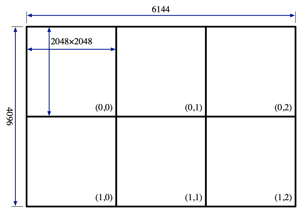
The cells of the grid are indexed by \((\mathit{row},\mathit{column})\) pairs, with the north-west cell having index \((0,0)\).

A map is represented in the file system as a directory. In the directory is a JSON file map.json that documents various properties of the map. For example, here is the map.json file from a map for the Grand Canyon:

{
    "name" : "Grand Canyon",
    "h-scale" : 60,
    "v-scale" : 10.004,
    "base-elev" : 284,
    "min-elev" : 414.052,
    "max-elev" : 2154.75,
    "min-sky" : 410,
    "max-sky" : 3000,
    "width" : 4096,
    "height" : 2048,
    "cell-size" : 2048,
    "color-map" : true,
    "normal-map" : true,
    "water-map" : false,
    "grid" : [ "00_00", "00_01" ]
}

The map information includes the horizontal and vertical scales (i.e., meters per unit); the base, minimum, and maximum elevation in meters; the upper limit of the skybox, the total width and height of the map in height-field samples;footnote:[ Note that the width and height are one less than the number of vertices; i.e., in this example, the number of vertices is \(4097\times 2049\). } the width of a cell; information about what additional data is available (color-map texture, normal-map texture, and water mask); and an array of the cell-directory names in row-major order. Each cell has its own subdirectory, which contains the data files for that cell. These include:

hf.png — the cell’s raw heightfield data represented as a 16-bit grayscale PNG file.
hf.cell — the cell’s heightfield organized as a level-of-detail chunks.
color.tqt — a texture quadtree for the cell’s color-map texture.
norm.tqt — a texture quadtree for the cell’s normal-map texture.
water.png — a 8-bit black and white PNG file that marks which of the cell’s vertices are water (black) and which are land (white).
objects.json — a list of object instances represented as a JSON array. The format of the JSON file follows that of Projects~3 and~4. The obj, mtl, and texture files for the objects will be in the map’s optional objects directory (to allow sharing across cells).^[1]

Of these files, the first four are guaranteed to be present, but water.png and objects.json are optional.

In addition to the cell subdirectories, if the map has objects on it, there will be an additional objects subdirectory to hold the obj, mtl, and texture files for the objects. Objects may have instances on multiple cells, which is why they are stored outside the cell subdirectories.

The sample code includes support for reading the map.json file, as well as the other data formats (.tqt and .cell files).

Because the map datasets can be quite large (some are in the 100’s of megabytes), we have only included some small examples in the GitHub repositories. The larger examples are available from the project webpage and will also be made available on the CSIL Macs.

Map Cell Files

The .cell files provide the key geometric information about the terrain being rendered. Each cell file consists of a complete quadtree of tiles (see cell.cpp for details on how a cell file is organized).

Each level of the quad tree defines a different level of detail and consists of \(2^{\textit{lod}} \times 2^{\textit{lod}}\) tiles arranged in a square grid. The tiles are indexed by their level, row, and column. A tile covers a square region of the cell and contains various bits of information, including a chunk, which is the triangle mesh for that part of the cell’s terrain at the tile’s level of detail.

Chunks are represented as a vertex array and an array of indices. The triangle meshes have been organized so that they can be rendered as triangle strips (VK_PRIMITIVE_TOPOLOGY_TRIANGLE_STRIP). Vertices in the mesh are represented as

struct Vertex {
    int16_t     _x;           // x coordinate relative to Cell's NW
                              // corner (in hScale units)
    int16_t     _y;           // y coordinate relative to Cell's base
                              // elevation (in vScale units)
    int16_t     _z;           // z coordinate relative to Cell's NW
                              // corner (in hScale units)
    int16_t     _morphDelta;  // y morph target relative to _y (in
                              // vScale units)
};

Note that the \(x\) and \(z\) coordinates of a vertex are relative the the cell’s coordinate system, not the world coordinate system. For large terrains, using single-precision floating point values for world coordinates can cause loss of precision when the viewer is far from the world origin. One can avoid these problems by splitting out the translation from model (i.e., cell) coordinates to camera-relative coordinates from the rest of the model-view-projection transform. The transformation of the Vertex structure to camera-relative coordinates in the vertex shader is straightforward. If we assume that \(\langle{} x, y, z, m \rangle{}\) is the 4-element Vertex,^[2] we compute

\[ \mathbf{v} = \langle{} s_x x, s_y y + s_m m, s_z z \rangle{} + \mathbf{o}_{\textit{cell}}\]

where \(\mathbf{s} = \langle{}s_x, s_y, s_z, s_m\rangle{}\) is a scaling vector and \(\mathbf{o}_{\textit{cell}}\) is the camera-relative origin of the cell (\(\mathbf{s}\) and \(\mathbf{o}_{\textit{cell}}\) are both uniform variables in the shader). The fourth component of the vertex is used to compute the vertex’s morph target, which is the projected position of the vertex in the next-lower level of detail. As described in \secref{sec:vertex-morph} below, the morph delta (\(m\)) is used to offset the altitude of the vertex (the adjusted altitude is called the morph target). Notice that \(\mathbf{v}\) is in a space where the axes are aligned with the world-space axes, but the origin is at the camera.

The chunk data structure also contains the chunk’s geometric error in the Y direction, which is used to compute screen-space error, and the chunk’s minimum and maximum Y values, which can be used to determine the chunk’s AABB.

The mesh data in a chunk is draw using triangle strips (see buffer-cache.hpp) and we use Vulkan’s primitive restart mechanism to enable the joining of disjoint meshes into a single drawing call (the mesh is actually five separate meshes: one for the terrain and four skirts). Your rendering code should enable primitive restart and set the restart value to 0xffff, which can be done the the following code. Note that primitive restart should be disabled after drawing the cell meshes, since it might break other drawing in your code.

\subsection{Texture Quad Trees} For each map cell, there are also two texture quad trees (TQTs) for the cell’s color and normal maps. TQTs provide a parallel structure to the tile quad tree and use the same indexing scheme. Support for loading texture quads from the file system is included as part of the common code.

1. We include support for adding objects to a map in the sample code for your use in Part 2 of the project, but you are free to ignore them.

2. The vertex fetch on the GPU will convert the 16-bit integers to floats.