Class Meeting 06: Measurement Models for Range Finders

Today's Class Meeting

Learning about two measurement models for range finders (Beam Models and Likelihood Fields), here's a link to today's slides
Implementing the likelihood field for range finders algorithm on the Turtlebot3

What You'll Need for Today's Class

For today's class, you'll need the following tools/applications ready and running:

Your Ubuntu 20.04 programming environment
Your particle filter localization project partner

Beam Models of Range Finders

Here, we detail a beam model for range finders algorithm.

$\textrm{Algorithm beam_range_finder_model}(z_t, x_t, m):$
$ \qquad q = 1 $
$ \qquad \textrm{for} \: k = 1 \: \textrm{to} \: K \: \textrm{do} $
$ \qquad\qquad \textrm{compute} \: z_t^{k*} \: \textrm{for the measurement} \: z_t^{k} \: \textrm{using ray casting} $
$ \qquad\qquad p = z_{hit} \cdot p_{hit}(z_t^k|x_t,m) + z_{short} \cdot p_{short}(z_t^k|x_t,m) + z_{max} \cdot p_{max}(z_t^k|x_t,m) + z_{rand} \cdot p_{rand}(z_t^k|x_t,m) $
$ \qquad\qquad q = q \cdot p$
$ \qquad \textrm{return} \: q $

Here, we provide additional details on the algorithm above:

$ z_t $ represents the laser range finder measurements received by the robot where $ z_t^k $ represents the $ k$-th range finder measurement
$ z_t^{k*}$ represents the "true" sensor measurement the robot would have read if it had been in the location we believe it to be in (i.e., the particle sensor measurement)
$ x_t $ represents the location we believe we are in (i.e., the particle location)
$ m $ represents the map of the world
the algorithm line $ q = q \cdot p $ comes from the way we incorporate all of the $K$ readings from the laser range finder, $p(z_t|x_t,m) = \prod_{k=1}^K p(z_t^k|x_t,m)$
$ (z_{hit} + z_{short} + z_{max} + z_{rand}) = 1 $

Accounting for possible measurement error in beam models

The beam model of range finders accounts for 4 types of possible measurement error: measurement noise, unexpected objects, failure to detect obstacles, and random measurements.

Measurement noise is accounted for through $ p_{hit}(z_t^k | x_t, m) $ according to: $$p_{hit}(z_t^k | x_t, m) = \{ \: \eta \mathcal{N}(z_t^k;z_t^{k*},\sigma_{hit}^2), \:\: \textrm{if} \: 0 \le z_t^k \le z_{max} \: ; \: 0, \: \textrm{otherwise} \}$$ where $\mathcal{N}(z_t^k;z_t^k*,\sigma_{hit}^2)$ denotes the univariate normal distribution with mean $z_t^{k*}$ and standard deviation $\sigma_{hit}$, and $\eta$ is a normalizing constant.

Unexpected objects (e.g., a person walking through the space that isn't captured in our static map) is accounted for through $ p_{short}(z_t^k | x_t, m)$ according to: $$p_{short}(z_t^k | x_t, m) = \{ \: \eta \lambda_{short} e^{-\lambda_{short}z_t^k}, \:\: \textrm{if} \: 0 \le z_t^k \le z_t^{k*} \: ; \: 0, \: \textrm{otherwise} \} $$ where $\lambda_{short}$ is an intrinsic parameter of the measurement model, and $\eta$ is a normalizing constant.

We account for a possible failure to detect obstacles assuming that failures result in a max-range measurement (due to, for example, sensing black light-absorbing objects or measuring objects in bright sunlights) according to: $$p_{max}(z_t^k | x_t, m) = \{ \: 1 \: \textrm{if} \: z = z_{max}, \: 0 \: \textrm{otherwise} \: \}$$

Finally, we account for random measurements according to: $$p_{rand}(z_t^k | x_t, m) = \{ \: \frac{1}{z_{max}} \textrm{if} \: 0 \le z_t^k \le z_{max}, \: 0 \: \textrm{otherwise} \: \}$$

Likelihood Fields for Range Finders

Here, we detail a likelihood field for range finders algorithm.

$ \textrm{Algorithm likelihood_field_range_finder_model}(z_t, x_t, m): $
$ \qquad q = 1 $
$ \qquad \textrm{for} \: k = 1 \: \textrm{to} \: K \: \textrm{do} $
$ \qquad \qquad \textrm{if} \: z_t^k \ne z_{max} $
$ \qquad \qquad \qquad x_{z_t^k} = x + x_{k,sens} cos \theta - y_{k,sens} sin \theta + z_t^k cos \big( \theta + \theta_{k,sens} \big) $
$ \qquad \qquad \qquad y_{z_t^k} = y + y_{k,sens} cos \theta - x_{k,sens} sin \theta + z_t^k sin \big( \theta + \theta_{k,sens} \big) $
$ \qquad \qquad \qquad dist = \textrm{min}_{x', y'} \: \Big\{ \sqrt{(x_{z_t^k} - x')^2 + (y_{z_t^k} - y')^2} \Big| \langle x', y' \rangle \: \textrm{occupied in } m \Big\} $
$ \qquad \qquad \qquad q = q \cdot \bigg( z_{hit} \: \textrm{prob}(dist,\sigma_{hit}) + \frac{z_{random}}{z_{max}} \bigg) $
$ \qquad \textrm{return} \: q $

Here, we provide additional details on the algorithm above:

$ z_t $ represents the laser range finder measurements received by the robot where $ z_t^k $ represents the $ k$-th range finder measurement and $ z_{max} $ represents the maximum possible value of the range finder
$ x_t = (x, y, \theta)^T$ represents the location we believe we are in (i.e., the particle location)
$ m $ represents the map of the world
$x_{k,sens}$, $y_{k,sens}$, and $\theta_{k,sens}$ represent the the location and orientation of the robot's sensor relative to the robot's position and heading (for our Turtlebot3, we can make the assumption that $x_{k,sens} = 0$ and $y_{k,sens} = 0$ ).
$\textrm{prob}(dist,\sigma_{hit}) $ is a zero-centered Gaussian with a standard deviation of $\sigma_{hit}$, where a zero-centered Gaussian distribution can be represented as $ g(x) = \frac{1}{\sigma{ \sqrt (2 \pi)}} e^{-x^2/2 \sigma^2} $
the algorithm line $ q = q \cdot \bigg( z_{hit} \: \textrm{prob}(dist,\sigma_{hit}) + \frac{z_{random}}{z_{max}} \bigg) $ comes from the way we incorporate all of the $K$ readings from the laser range finder, $p(z_t|x_t,m) = \prod_{k=1}^K p(z_t^k|x_t,m)$
$ (z_{hit} + z_{max} + z_{rand}) = 1 $

Class Exercise: Likelihood Field in 4 Directions for the Turtlebot3

Today's class exercise will give us an opportunity to implement the likelihood field algorithm with our Turtlebot3 in the Gazebo simulated house environment. For this exercise, please work with your particle filter project partner.

Getting Started

To get started on this exercise, update the intro_robo class package to get the class_meeting_06_likelihood_field ROS package and starter code that we'll be using for this activity.

$ cd ~/catkin_ws/src/intro_robo
$ git pull
$ git submodule update --init --recursive
$ cd ~/catkin_ws && catkin_make
$ source devel/setup.bash

Running your code

First terminal: run roscore.

$ roscore

Second terminal: run your Gazebo simulator with the Turtlebot3 house environment.

$ roslaunch turtlebot3_gazebo turtlebot3_house.launch

Third terminal: launch the launchfile that we've constructed that starts up the map server and runs rviz with some helpful configurations already in place for you (visualizing the map, particle cloud, robot location). If the map doesn't show up when you run this command, we recommend shutting down all of your terminals (including roscore) and starting them all up again in the order we present here.

$ roslaunch class_meeting_06_likelihood_field visualize_particles.launch

Fourth terminal: run the python node that runs the likelihood field algorithm (measurement_update_likelihood_field.py is the file that you'll be working in for this exercise - we've provided some starter code in this file, do your exercise in the section marked TODO).

$ rosrun class_meeting_06_likelihood_field measurement_update_likelihood_field.py

Your goal

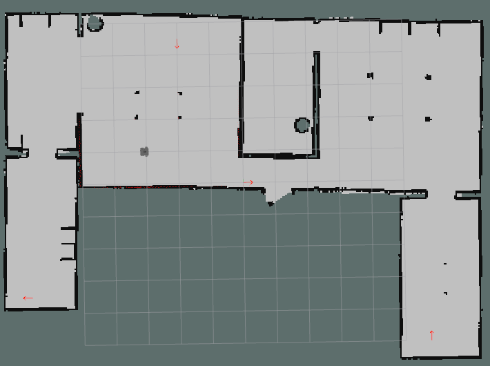
Your goal in this exercise is to implement the likelihood field measurement model algorithm for your Turtlebot3 in the house environment for 4 particles, using only 4 of the 360 range finder values (0, 90, 180, 270). Using a small number of particles and a subset of the laser range finder values will enable us to more easily debug and get a sense of how the algorithm works before scaling up. When you run your code, you should see the four particles in your RViz window:

For each particle, compute the importance weight according the likelihood_field_range_finder_model algorithm detailed above with one small change to make things just a bit simpler for this exercise. Instead of $$q = q \cdot \bigg( z_{hit} \: \textrm{prob}(dist,\sigma_{hit}) + \frac{z_{random}}{z_{max}} \bigg)$$ we will implement this step as $$q = q \cdot \textrm{prob}(dist,\sigma_{hit}) $$ If you would like to implement the likelihood field algorithm using $q = q \cdot \big( z_{hit} \: \textrm{prob}(dist,\sigma_{hit}) + \frac{z_{random}}{z_{max}} \big) $ for your particle filter project, please do! For the purposes of this exercise, though, we'll stick with the simpler version.

The Starter Code

There are a few methods that I'd like to draw your attention towards as you work on this exercise:

get_closest_obstacle_distance(x,y) in the file likelihood_field.py takes in a location on the map and returns the distance to the closest obstacle to that point (e.g., a wall, a bookshelf, a table leg). The code in likelihood_field.py computes the likelihood field ahead of time (see the __init__ method) so that you don't have to re-compute it each time you want to compute the closest obstacle to a particular (x,y) point in the world.
compute_prob_zero_centered_gaussian(dist, sd) is a method that computes the Gaussian function for the distance between the robot's measurement and the closest obstacle to the particle's sensor measurement given a standard deviation (I used a value of 0.1 for the standard deviation for this class exercise). This method is meant to implement $\textrm{prob}(dist,\sigma_{hit})$.
The methods euler_from_quaternion() and quaternion_from_euler() can transform the orientation of the particles/robot from quaternion to Euler angles and back. These are built in Python functions from the tf.transformations library.

Application to Your Particle Filter Project

You are more than welcome to use the code you develop today and the code we provide (especially likelihood_field.py) in your particle filter project implementation.

Checking Your Solution

This section contains solution values for the likelihood field in 4 directions for this exercise. Please note that due to noise in Gazebo, your values may slightly differ from those listed below.

Particle at location [0.0, 0.0, 0.0]

Laser Scan Index	Laser Scan Value $(z_t^k)$	Projected Scan Location $ \big[ x_{z_t^k}, y_{z_t^k} \big] $	Distance to Nearest Obstacle $(dist)$	$\textrm{prob}(dist,\sigma_{hit})$ where $\sigma_{hit} = 0.1$
0	2.87	[2.87, 0.0]	0.20	0.54
90	3.5 (max)	[0.0, 3.5]	0.0	3.99
180	2.08	[-2.08, 0.0]	0.05	3.52
270	1.10	[0.0, -1.10]	0.85	8.16e-16

Particle at location [-6.6, -3.5, $\pi$]

Laser Scan Index	Laser Scan Value $(z_t^k)$	Projected Scan Location $ \big[ x_{z_t^k}, y_{z_t^k} \big] $	Distance to Nearest Obstacle $(dist)$	$\textrm{prob}(dist,\sigma_{hit})$ where $\sigma_{hit} = 0.1$
0	2.87	[-9.47, -3.50]	2.00	5.52e-87
90	3.5 (max)	[-6.60, -7.00]	3.15	1.37e-215
180	2.08	[-4.52, -3.50]	0.70	9.13e-11
270	1.10	[-6.60, -2.40]	0.80	5.05e-14

Particle at location [5.8, -5.0, $\pi/2$]

Laser Scan Index	Laser Scan Value $(z_t^k)$	Projected Scan Location $ \big[ x_{z_t^k}, y_{z_t^k} \big] $	Distance to Nearest Obstacle $(dist)$	$\textrm{prob}(dist,\sigma_{hit})$ where $\sigma_{hit} = 0.1$
0	2.87	[5.80, -2.13]	0.67	5.96e-10
90	3.5 (max)	[2.30, -5.00]	2.55	2.52e-141
180	2.08	[5.80, -7.08]	1.50	5.53e-49
270	1.10	[6.90, -5.00]	0.40	0.0013

Particle at location [-2.0, 4.5, $-\pi/2)$]

Laser Scan Index	Laser Scan Value $(z_t^k)$	Projected Scan Location $ \big[ x_{z_t^k}, y_{z_t^k} \big] $	Distance to Nearest Obstacle $(dist)$	$\textrm{prob}(dist,\sigma_{hit})$ where $\sigma_{hit} = 0.1$
0	2.87	[-2.00, 1.63]	0.40	0.0012
90	3.5 (max)	[1.50, 4.50]	0.55	1.08e-06
180	2.08	[-2.00, 6.58]	1.30	8.00e-37
270	1.10	[-3.10, 4.50]	0.75	2.15e-12

Solution Code

We will NOT be giving out solution code for this exercise. If you have questions about your implementation or would like to get help on this exercise, please reach out to the teaching staff and/or attend our office hours. We'd be more than happy to help!

Acknowledgments

This page and the content for today's lecture were informed by Probabilistic Robotics by Sebastian Thrun, Wolfram Burgard, and Dieter Fox.