Class Meeting 07: Markov Decision Processes (MDPs)

Today's Class Meeting

Learning about Markov decision processes (here's a link to the slides)
Completing hands-on exercises computing & determining Markov decision process policies and values; on this page you can find solutions to the class exercises

What You'll Need for Today's Class

Some scratch paper to work through some of today's class exercises

Markov Decision Process (MDP)

A Markov decision process (MDP) is defined by the tuple \( \langle S, A, T, R, \gamma \rangle \), where:

\(S\) is the set of possible states with \(s \in S\)
\(A\) is the set of possible actions that can be taken \(a \in A\), in our case, these are usually the actions that the robot can take
\(T: S \times A \times S \rightarrow [0,1]\) is a probabilistic transition function where \(T(s_t, a_t, s_{t+1}) \equiv \textrm{Pr}(s_{t+1} | s_t, a_t)\), representing the probability that we end up in state \(s_{t+1}\) given that we started in state \(s_t\) and took action \(a_t\)
\(R: S \times A \times S \rightarrow \mathbb{R}\), the reward function where a \((s_t, a_t, s_{t+1})\) tuple is assigned a real-number (\(\mathbb{R}\)) reward value
\(\gamma\) is the discount factor where \((0 \le \gamma \lt 1) \), which indicates how much future rewards are considered in the actions of a system
- \(\gamma = 0\) would indicate a scenario in which a robot only cares about the rewards it could get in a single moment, as where
- \(\gamma = 1\) indicates a scenario where the robot doesn't care at all about the short term and pursues whatever actions will produce the best long-term reward (regardless of how long that takes)

Additionally, we can compute

\(\pi(s_t) \rightarrow a_t\), a policy that determines an optimal action to take for every state in the state space
\(V(s_t)\), the value of being in a state given by the Bellman equation where \(V(s_t) = \textrm{max}_{a_t} \Bigg( R(s_t,a_t) + \gamma \sum_{s_{t+1} \in S} T(s_t, a_t, s_{t+1}) \: V(s_{t+1}) \Bigg)\)

For today's class the environment we're exploring is a grid world, pictured below.

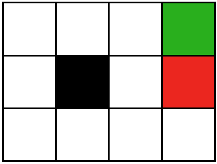
With this grid world, we define the following Markov decision process \( \langle S, A, T, R, \gamma \rangle \):

\(S\): our states are represented as grid cells, each grid cell is one state in our world
\(A\): the actions the robot can take in the world include moving up, down, left, and right; so there are 4 total actions that can be taken in this world
\(T\): the robot moves as expected with action \(a_t\) from one state (\(s_t\)) to another (\(s_{t+1}\)) with probability 0.8. With probability 0.1, the robot moves as intended except to the right. And with probability 0.1, the robot moves as intended except to the left. Here are some examples:
- If \(a_t\) specifies that the robot should move to the right, with probability 0.8 the robot will move right. With probability 0.1 the robot will move up. And with probability 0.1 the robot will move down.
- If \(a_t\) specifies that the robot should move down, with probability 0.8 the robot will move down. With probability 0.1 the robot will move right. And with probability 0.1 the robot will move left.
Additionally, the robot cannot move outside the boundaries of the world. If the robot tries to get outside the boundary, it will end up in the exact same place it started in such that (\(s_{t+1} = s_t\)). Lastly, if the robot ends up in either the red or green grid cells, the game ends.
\(R\): for today's class we only depend on the state of the world to determine the reward, the reward for being in the green square is \(+1\) and the reward for being in the red square is \(-1\), the reward for being in the remaining states depends on the exercise
\(\gamma\): for today's class we'll use a gamma value of 0.8

Class Exercise #1: Determining MDP Policies with Different Reward Functions

For this exercise, you will determine the optimal policy for the grid world with two different reward functions. For each reward function, you will determine a unique optimal policy.

Reward function #1:

\(R(\textrm{green}) = +1\)
\(R(\textrm{red}) = -1\)
\(R(\textrm{everywhere else}) = +2\)

Reward function #2:

\(R(\textrm{green}) = +1\)
\(R(\textrm{red}) = -1\)
\(R(\textrm{everywhere else}) = -2\)

Note: You can find the solutions on this page.

Class Exercise #2: Value Iteration Computation

For today's class exercise, please get together in groups of 2-3 students.

Value Iteration

With our grid world and the specified reward function (which is the same as reward function #2 from exercise #1), compute the value for each state in the grid world using the Bellman equation: \(V(s_t) = \textrm{max}_{a_t} \Big( R(s_t,a_t) + \gamma \sum_{s_{t+1} \in S} T(s_t, a_t, s_{t+1}) \: V(s_{t+1}) \Big)\) and the value iteration approach. Before we start with value iteration, you can assume that the value for each state is 0.

Reward function:

\(R(\textrm{green}) = +1\)
\(R(\textrm{red}) = -1\)
\(R(\textrm{everywhere else}) = -2\)

Note: To best keep track of each state, we will denote each state by it's row and column where the bottom left is the origin [0,0]. For example, the green state at time \(t\) can be represented as \(s_t = [2,3]\)

To keep everyone on the same page, we're all going to follow the same set of trajectories:

	Trajectory 1	Trajectory 2	Trajectory 3	Trajectory 4	Trajectory 5	Trajectory 6
\(s_0\)	[0,0]	[0,0]	[0,0]	[0,0]	[0,0]	[0,0]
\(a_0\)	UP	UP	RIGHT	RIGHT	UP	RIGHT
\(s_1\)	[1,0]	[1,0]	[0,1]	[0,1]	[1,0]	[0,1]
\(a_1\)	UP	UP	RIGHT	RIGHT	UP	RIGHT
\(s_2\)	[2,0]	[2,0]	[0,2]	[0,2]	[2,0]	[0,2]
\(a_2\)	RIGHT	RIGHT	UP	RIGHT	RIGHT	UP
\(s_3\)	[2,1]	[2,1]	[1,2]	[0,3]	[2,1]	[1,2]
\(a_3\)	RIGHT	RIGHT	RIGHT	UP	RIGHT	UP
\(s_4\)	[2,2]	[2,2]	[1,3]	[1,3]	[2,2]	[2,2]
\(a_4\)	RIGHT	RIGHT			RIGHT	RIGHT
\(s_5\)	[2,3]	[2,3]			[2,3]	[2,3]

To get a better sense of how to attack this problem, we'll help you out by computing the values for the first trajectory and the first two steps of the second trajectory:

Trajectory 1

\(V([2,3]) = +1\)
- We can determine this value because \(R(s_t,a_t) = +1\) for being in the green state and once we get into the green state, the world ends (we cannot transition into any further states), meaning that for all \(a_t\), \(\Big(\gamma \sum_{s_{t+1} \in S} T(s_t, a_t, s_{t+1}) \: V(s_{t+1}) \Big) = 0\).
\(V(\textrm{all-other-states}) = -2\)
- We can determine this value because \(R(s_t,a_t) = -2\) and all states initially starts out with a value of 0, \(V(s_{t+1}) = 0\), for all states until after we go through the first iteration.

Trajectory 2

\(V([0,0]) = -2 + \gamma (0.8 \cdot 0 + 0.1 \cdot -2 + 0.1 \cdot -2) = - 2 + \gamma (-0.4) = -2 + 0.8 \cdot -0.4 = -2.32\)
- The optimal action in this case would be a move to the RIGHT, since the value of state [0,1] is currently 0 and the value of state [1,0] is currently -2.
\(V([1,0]) = -2 + \gamma (0.8 \cdot -2 + 0.1 \cdot -2 + 0.1 \cdot -2) = -2 + \gamma (-2) = -2 + 0.8 \cdot -2 = -3.6 \)
- The optimal action in this case would be a move UP since the value of state [2,0] is currently -2 and the value of state [0,0] is currently now -2.32.

Note: You can find the solutions on this page.

Acknowledgments

The lecture for today's class was informed by Kaelbling et al. (1996) and Charles Isbell and Michael Littman's Udacity course on Reinforcement Learning.