Class Meeting 07: Path Finding

Today's Class Meeting

Learning about path finding algorithms, reviewing value iteration and learning the A* algorithm - here's a link to the slides
Completing a hands-on exercise, executing the A* algorithm for a grid world example

Value Iteration

\(\textrm{Algorithm MDP_discrete_value_iteration}():\)
\( \qquad \textrm{for} \: s \in S \: \textrm{do} \)
\( \qquad\qquad V(s) = min\big(R(s_t, a_t)\big) \)
\( \qquad \textrm{repeat until convergence} \)
\( \qquad \qquad \textrm{for} \: s \in \{s_0, s_1, s_2, ... \} \: \textrm{do} \)
\( \qquad\qquad\qquad V(s_t) = \textrm{max}_{a_t} \Big( R(s_t,a_t) + \gamma \sum_{s_{t+1} \in S} T(s_t, a_t, s_{t+1}) \: V(s_{t+1}) \Big)\)
\( \qquad \textrm{return} \: V \)

For this algorithm, we assume that we are working with a Markov decision process \( \langle S, A, T, R, \gamma \rangle \), where

\(s \in S\) represents the states in our world and \(\{s_0, s_1, s_2, ... \}\) represents a single trajectory a robot may traverse
\(a \in A\) represents the actions the robot can take in the world
\(T(s_t, a_t, s_{t+1})\) is the transition function, where the robot moves as expected with action \(a_t\) from one state (\(s_t\)) to another (\(s_{t+1}\)) with specified probabilities
\(R(s_t, a_t)\) is the reward function
\(\gamma\) is the discount factor

Once we have completed the value iteration process, we can now specify an optimal policy for selection actions based on our converged value function (\(V^*\)) as we can see from the algorithm below.

\(\textrm{Algorithm execute_MDP_policy}(x, V^*): \)
\( \qquad \textrm{return} \: \: \underset{a_t}{\textrm{argmax}} \:\Big[ R(s_t, a_t) + \gamma \sum_{s_{t+1} \in S} T(s_t, a_t, s_{t+1}) \: V^*(s_{t+1}) \Big] \)

A* Pathfinding Algorithm

The A* pathfinding algorithm can be used to find the most efficient path from a start location to a goal location. The A* algorithm makes the following significant assumptions:

you know the map of the environment
the environment can be represented as a graph
you know the location of the robot's start position
you know the location of the robot's goal location

The A* algorithm computes the following terms for nodes, \(n\) in the graph:

\(g(n)\) - the movement cost of the path from the start node to the current node (\(n\))
\(h(n)\) - the estimated movement cost of hte path from the goal node to the current node (\(n\))
\(f(n) = g(n) + h(n)\)

The A* algorithm is implemented as follows:

Initialize the open set to a queue with only the start node within it
Until the goal node is removed from the open set, do the following:
- Set the next current node to be the node in the open set with the lowest \(f\)-value
- Remove the current node from the open set
- Compute/update the \(f\)-values for all of the current node's neighbors
- Add all of the current node's neighbors to the open set queue

A Grid World Example

In class lecture, we cover the following example grid world. We assume that the movement cost of moving one grid cell up, right, down, and left is 10 units. We assume that moving diagonally has a movement cost of 14 units.

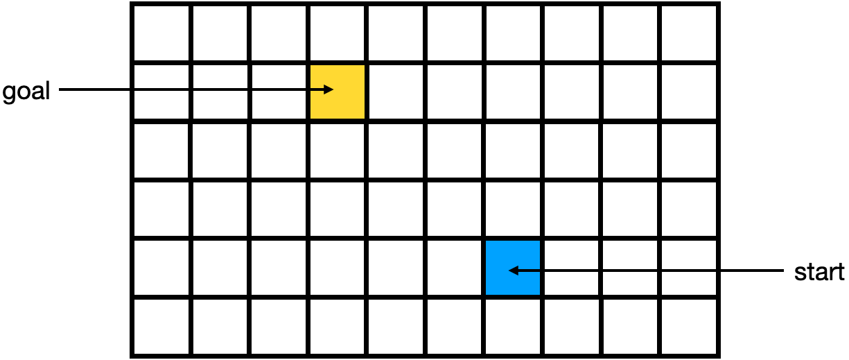
The algorithm starts with the start node. We compute the \(g\), \(h\), and \(f\) values for each of the neighbors of the start node. In the diagram below, you can find the \(g\) value in the upper left corner of each grid cell, the \(h\) value in the upper right corner of each grid cell, and the \(f\) value in the center of each grid cell.

Our next current node will be the node with the \(f\) value of 42. We will next compute the \(g\), \(h\), and \(f\) values for each of its neighbors.

The upper left neighbor of the current node has the lowest \(f\) value (still 42), so we will select it to be our next current node, computing the \(g\), \(h\), and \(f\) values for each of its neighbors.

Finally, we select the upper left node as the next current node, and we are happy to find that it is the end node! We can stop the algorithm. Now we have a best path from start to end with a final movement cost, \(f\)-value, of 42.

Class Exercise: A* Algorithm for a Grid World with Obstacles

Please work in a group of 2-3 students for this exercise. We will execute the rest of the A* algorithm on the same grid world, but this time, we have an obstacle.

Note: You can find the solution to this exercise on this page.

Acknowledgments

The value iteration component of today's lecture was informed by Probabilistic Robotics by Sebastian Thrun, Wolfram Burgard, and Dieter Fox as well as Kaelbling et al. (1996) and Charles Isbell and Michael Littman's Udacity course on Reinforcement Learning. The A* algorithm content of today's class was informed by the A* wikipedia page as well as Sebastian Lague's YouTube video on A* Pathfinding. The lecture for today also features this YouTube video about the Shakey robot.