Schelling’s Model of Housing Segregation
Due: Friday, October 23, 3pm CDT
The goal of this assignment is to give you practice using nested loops, lists of lists, and functions.
You may work alone or in a pair on this assignment. The algorithms you need to implement for this assignment are more challenging than the first assignment. We recommend starting early.
Getting started
If you are going to work alone, before you start working on the
assignment’s tasks, please take a moment to follow the steps described
in Coursework Basics page to get the files for this assignment
(these steps will be the same as the ones you followed to get the
files for Short Assignment #1). Please note that you will not be able
to start working on the assignment until you fetch the assignment
files (which will appear in a pa2 directory in your repository)
If you are going to work in a pair, please follow the “Working in a Pair” instructions in Coursework Basics to get started.
Students working in pairs should NOT use their individual repositories
Please note that this means you will not be able to start working on the assignment until you request and setup your pair repository.
Introduction
The New York Times has an interesting tool for viewing the distribution of racial and ethnic groups in cities and states around the country. If you look at the map for the Greater Chicago area, you will see that many areas are heavily segregated, but that some, such as the suburb of Glendale Heights, are not. The forces that led to this arrangement of people are complex and it is unlikely that any simple model can truly answer the questions of how segregation arises and why it persists. Keeping that in mind, one can still ask simple questions that may shed some light on the situation. In his 1978 book Micromotive and Macrobehavior, Thomas Schelling considered the following question: is it possible that a group of individuals would prefer to live in integrated neighborhoods and yet, as the result of their collective choices end up in segregated neighborhoods?
Schelling examined this question using a very simple model: A city has two kinds of people, Cubs fans and White Sox fans, for example, and each person in the city requires a certain number of their neighbors to be like them to feel comfortable in their location. Schelling used this model to study the patterns that emerge if, over time, people who are unsatisfied with their initial locations or become unsatisfied over time relocate to new locations that satisfy their criteria. What happens depends on the ratio of the two populations and on the satisfaction criteria used by the individuals, but segregation is a frequent outcome.
Schelling’s model of housing segregation has led to myriad follow-up work examining different facets of the model’s outcomes in different circumstances, as well as applying the model to longitudinal datasets of urban environments. Data about Chicago features in a number of these analyses.
Our Model
Your task in this assignment will be to implement a variant of Schelling’s model. Before you can do so, we need to specify the details of the abstract model we will be using and then describe the concrete data structures we will be using to implement the model.
For the model, we need to specify, the:
shape and composition of a city,
boundaries of a home’s neighborhood,
definition for a similarity score,
definition for satisfaction,
rule for relocating homeowners,
composition of a relocation wave in the simulation,
composition of a step in the simulation, and
stopping conditions for the simulation.
Cities: A city is modelled as an \(N \times N\) grid (where the value of \(N\) can be different for each city). Each grid location (or cell) represents a home, which can be for sale, occupied by a maroon homeowner, or occupied by a blue homeowner. You may assume that a city has at least one home for sale and homes that are for sale are not occupied.
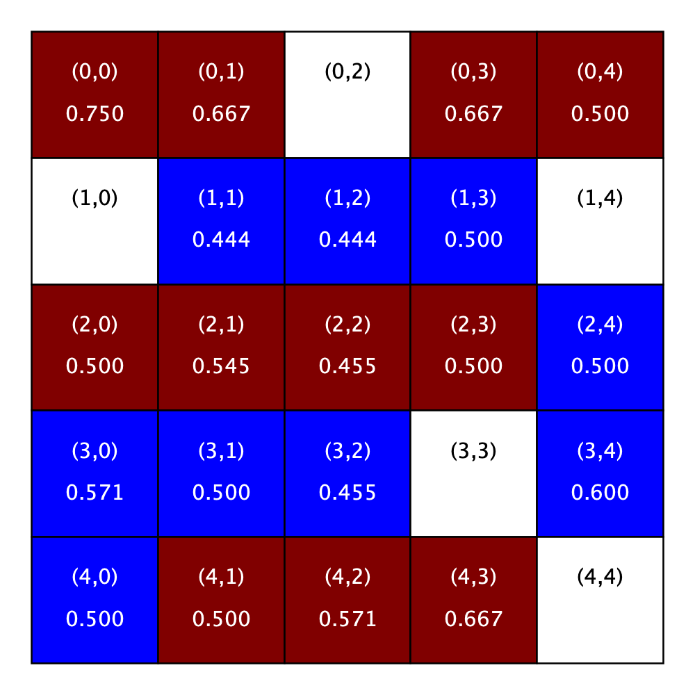
Here is a sample city that we will use throughout this write-up:
Sample City |
|---|
In this and in nearly all subsequent city depictions, a white cell indicates a home that is for sale, a maroon (dark red) cell indicates that a home is occupied by a maroon homeowner, and a blue cell indicates a home that is occupied by a blue homeowner. This figure also includes the location (in parentheses) of each home (cell) to help orient you in the city.
Neighborhood
The neighborhood of a home will be defined by a parameter R. The R-neighborhood of the home at Location (i,j) in an \(N \times N\) city contains all Locations (k,l) such that:
If you look carefully at the definition, you will note that Location (i,j) itself is considered part of its own neighborhood.
We will refer to a neighborhood with parameter R=x as an “R-x neighborhood”.
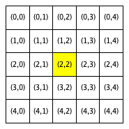
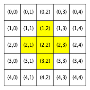
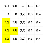
The following figures show the neighborhoods around Locations (2,2) and (3,0) for different values of R. In this set of figures (and this set only), we use yellow to indicate that a location is included in the specified neighborhood and white to indicate that a location is not included in the neighborhood.
Neighborhood around (2,2) |
Neighborhood around (3,0) |
||
|---|---|---|---|
R = 0 |
R = 1 |
R = 1 |
R = 2 |
Notice that Location (3,0), which is closer to the boundaries of the city, has fewer neighboring homes for the same value of R than Location (2,2), which is the middle of the city. We use the term boundary neighborhood to refer to a neighborhood that is near the boundary of the city and thus does not have a full set of neighbors.
Similarity score
We define the similarity score of a homeowner at a given location to
be S/H where S is the number of homes in the neighborhood
centered on that location with occupants of the same color as the
homeowner and H is the number of occupied homes in the
neighborhood.
Since a homeowner is included in their own neighborhood, S and
H will each be at least one, and so, a homeowner’s similarity
score will always be defined and will be greater than zero.
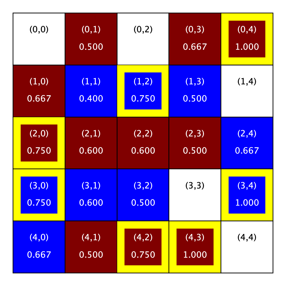
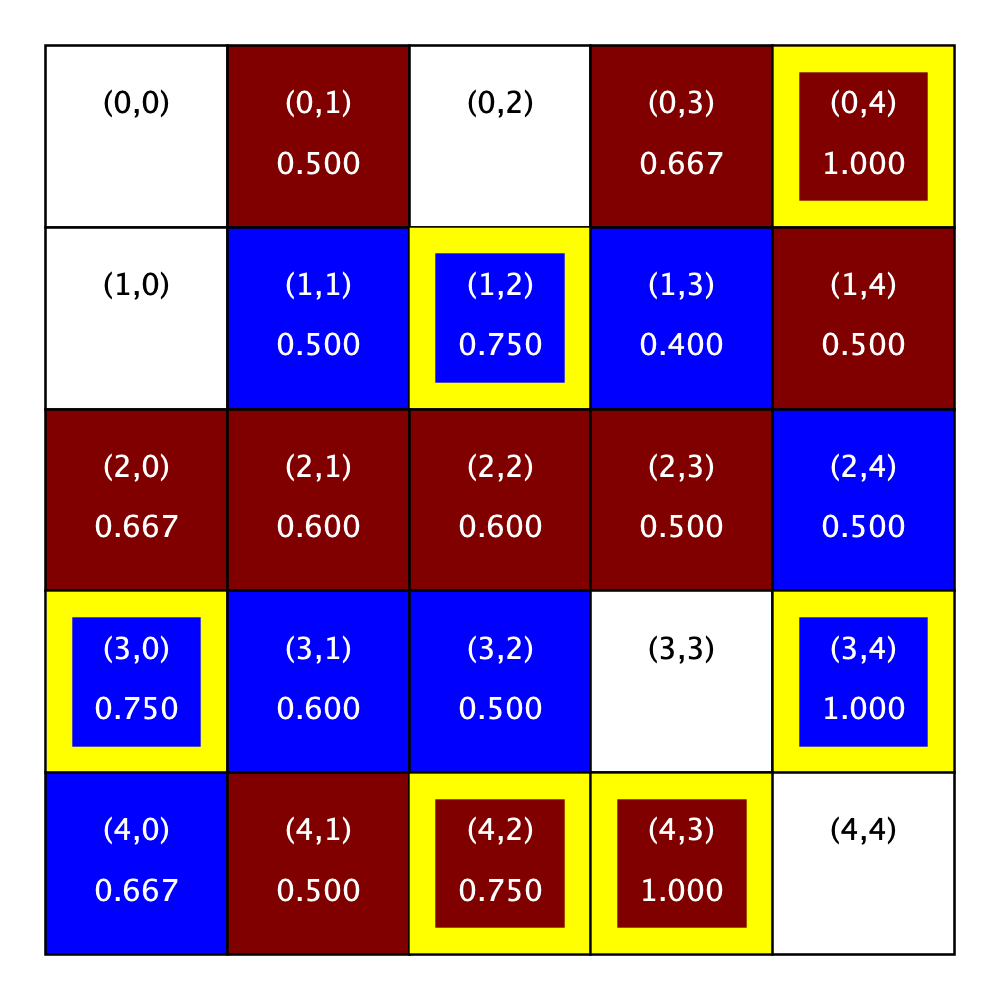
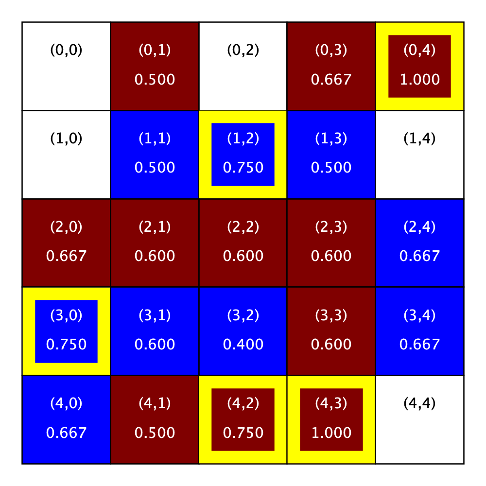
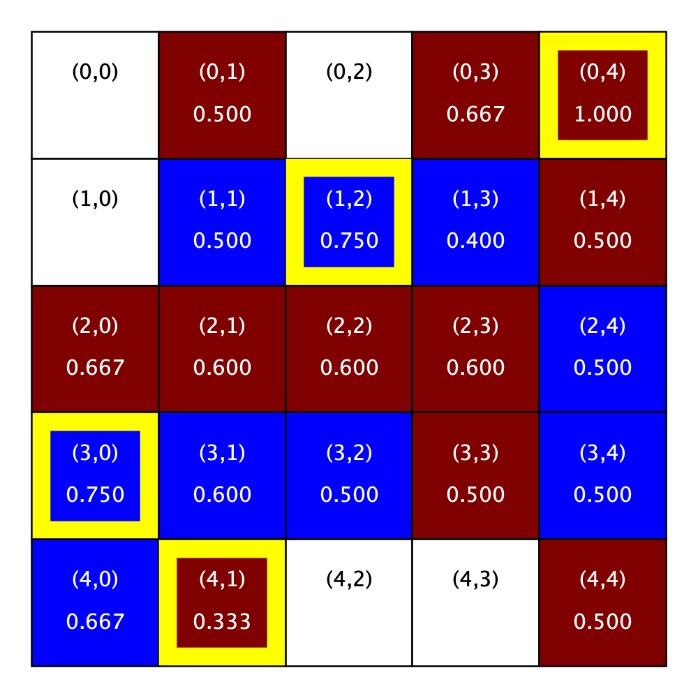
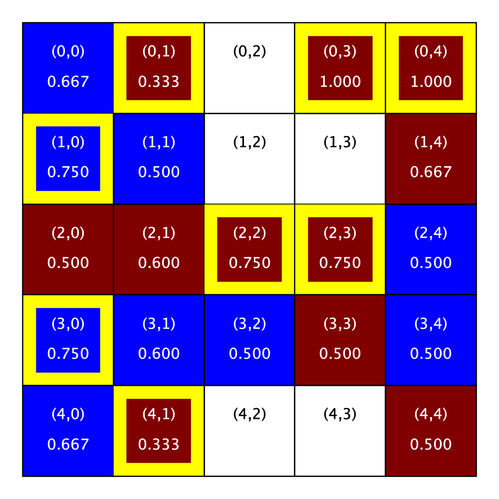
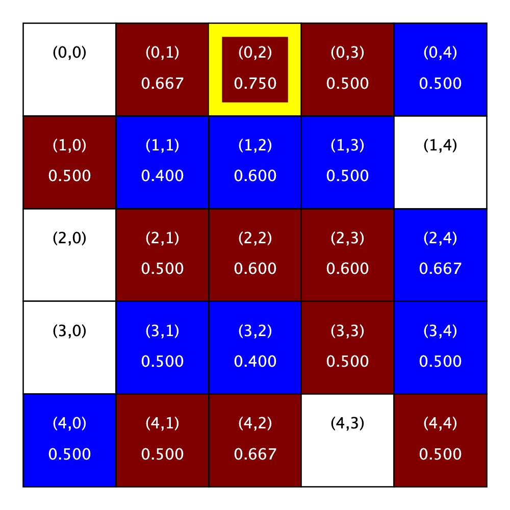
The figures below illustrate this concept using a the sample city shown above with R-1 neighborhoods (left) and R-2 neighborhoods (right). The similarity scores are shown beneath the location in each grid cell. Notice the figure does not include similarity scores for the homes that are for sale (that is, those that are shown in white), because they are unoccupied and it does not make sense to compute a similarity score for a home without a homeowner.
Similarity scores |
|
|---|---|
City parameters:
R: 1
|
City parameters:
R:2
|
Satisfaction
A homeowner is satisfied with their location if their similarity score falls within a specified range, inclusive of the end points of the range.
Ideally, we would allow different homeowners to use different ranges, but to simplify your task, we will use the same range for everyone in a city. The range will be a parameter to the simulation.
Why use a range? Because it allows us to simulate different levels of demand for integration (or segregation) across different runs of the simulation. To model a population that prefers integration, we might use a range of \([0.45, 0.55]\), whereas to simulate a more ambivalent population we could use \([0.20, 0.80]\).
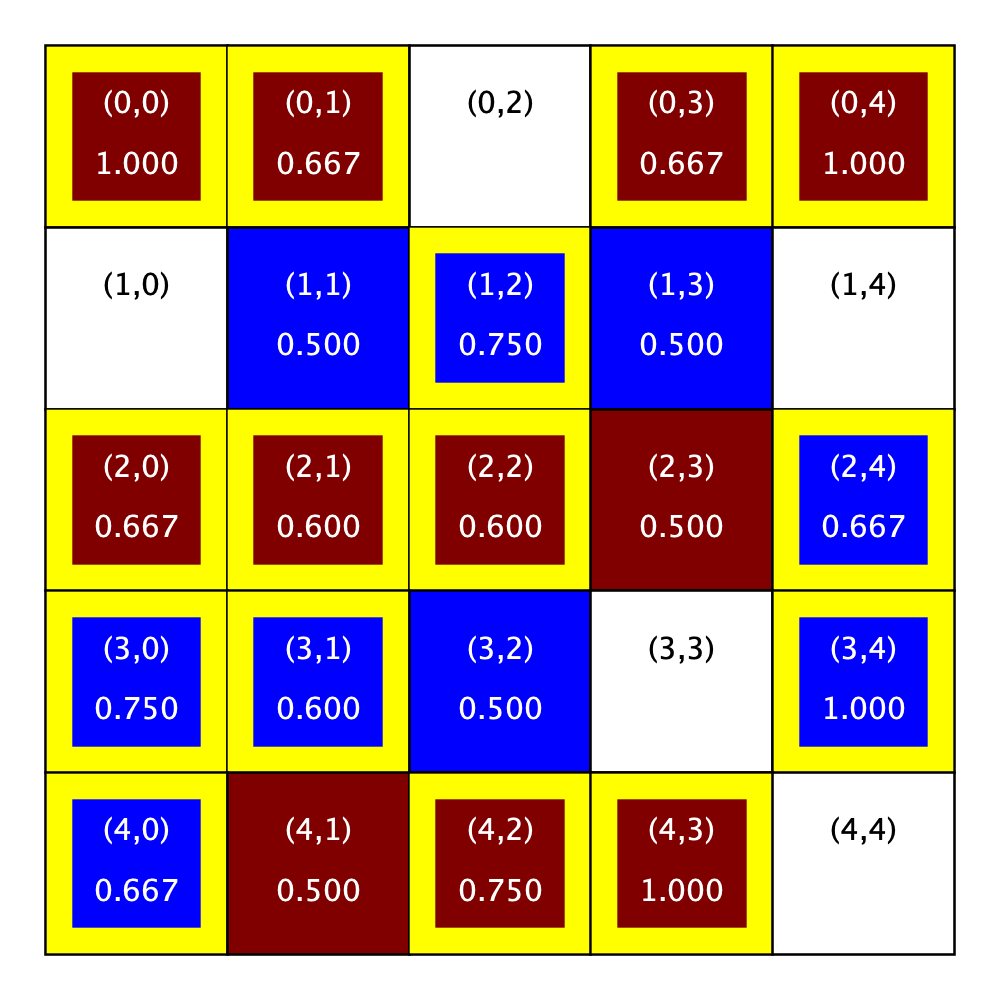
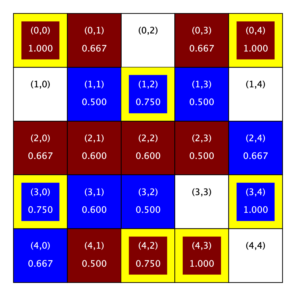
Let’s apply this definition of satisfaction to our sample R-1 neighborhood. The figure on the left uses satisfaction range of \([0.45, 0.55]\), while the figure on the right uses \([0.4, 0.7]\). Throughout this assignment, we indicate unsatisfied homeowners with a yellow border.
Satisfaction Examples |
|
|---|---|
City parameters:
R: 1
Satisfaction range: [0.45, 0.55]
|
City Parameters:
R: 1
Satisfaction range: [0.4, 0.7]
|
Notice that some of the people who were unsatisfied when the range was very narrow (\([0.45, 0.55]\)) are no longer unsatisfied once the range is expanded a bit (\([0.4, 0.7]\)).
Homes for sale
We will use an ordered list to keep track of the homes that are for sale. The initial ordering of the list the homes that are for sale is a parameter to the simulation. As our homeowners move around the city, homes that were for sale will come off the list and newly empty homes will be added to the list. Our homeowners prefer to consider homes that have recently come on the market first and so, newly empty homes will be added to the beginning of the list.
Relocation rule
Our homeowners want to live in satisfactory locations and will relocate when they are unsatisfied. We’ll describe how to relocate a specific homeowner and then talk about how to navigate through the city finding homeowners to relocate.
Homeowners will only move to homes in locations that are satisfactory. How do we decide whether a new location is satisfactory: we’ll temporarily swap the homeowner to the new location, apply the satisfaction rule to the new location, and then swap the homeowner back to their original location.
A city will always have at least one home available for sale at any given time and typically, will have many more than one for sale. How does the homeowner choose among multiple satisfactory homes? In real life, homeowners have lots of different criteria. In our simulation, everyone will use the same mechanism for picking a new home: they start out eager to check out new homes, but over time they will lose patience and just choose the next one that is satisfactory. We will model patience with a parameter that will be the same for everyone in the city. Homeowners will evaluate homes that are for sale in the order they appear in the list of homes for sale. The homeowner’s patience level starts out at the specified level and decreases every time they find a home that is satisfactory. As soon as their patience level hits zero, they stop looking and choose that home. If a homeowner evaluates all of the homes that are for sale and never gets to a patience level of zero, they will choose not to move.
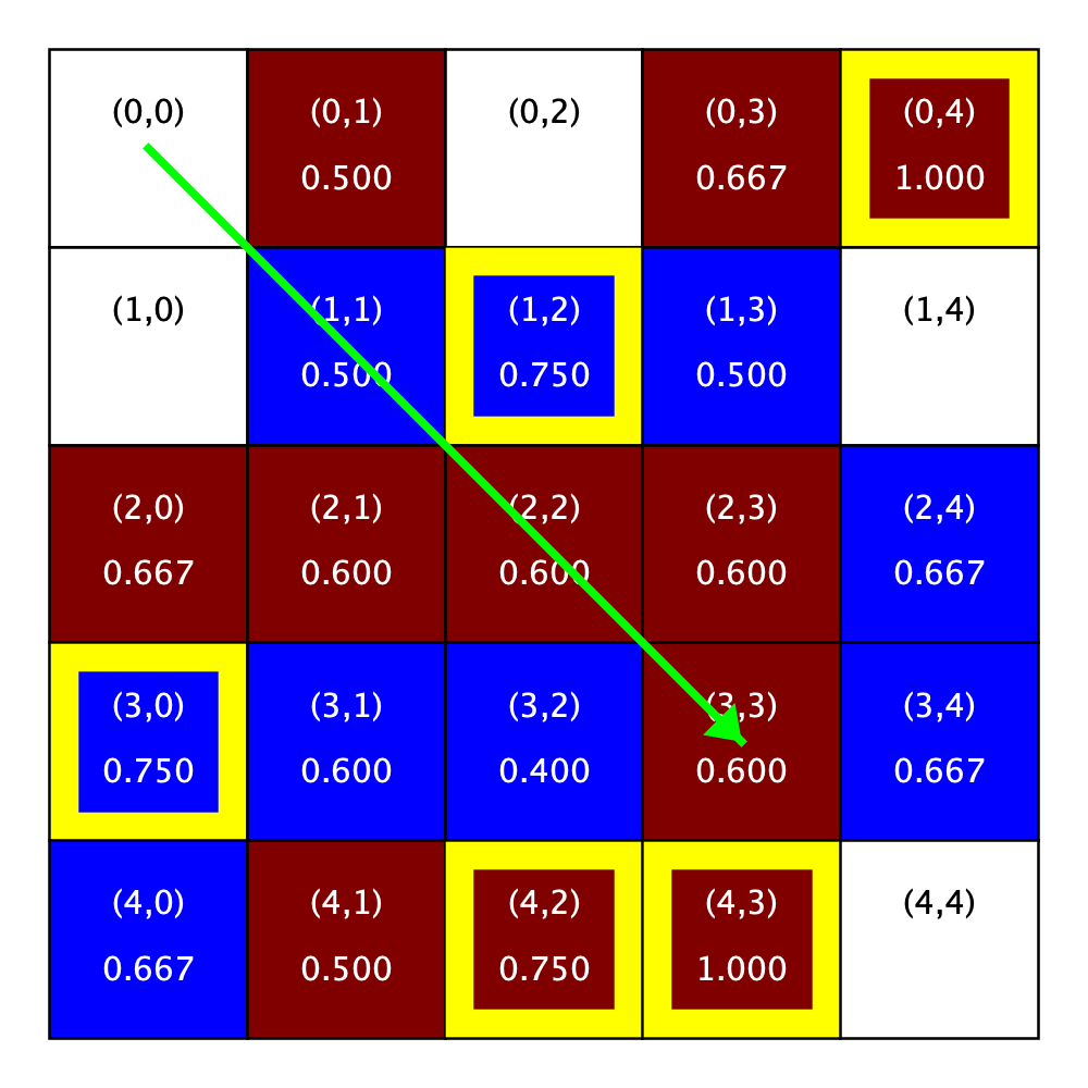
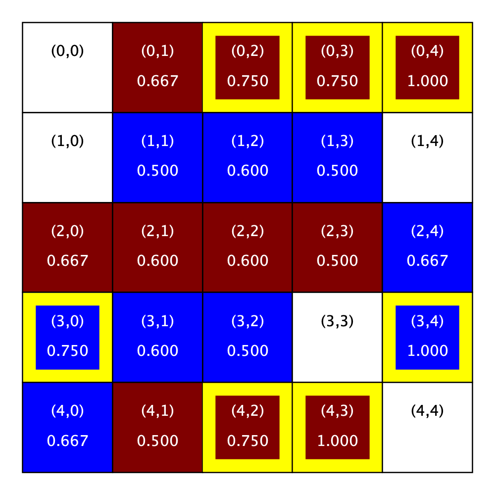
The figure below shows a city and the order of homes that are for sale before and after we relocate the homeowner in Location (0, 0).
Relocating the homeowner in Location (0, 0) |
|
|---|---|
City parameters
R: 1
Satisfaction range: [0.4, 0.7]
Patience level: 3
|
|
Let’s walk through the details of this relocation given the specified parameters for the city. Following the relocation rule, we will try relocating the homeowner to each of the homes that are for sale in turn until they run out of patience or we run out of homes.
Attempted relocations of the homeowner at Location (0, 0)
|
||
|---|---|---|
City parameters
R: 1
Satisfaction range: [0.4, 0.7]
Patience Level: 3
|
||
For Sale |
Temporary City |
Explanation |
Original grid with the (unsatisfied) homeowner in Location (0, 0). |
||
Location (0, 2) |
Homeowner is not satisfied in the home at Location (0, 2) |
|
Location (1,0) |
Homeowner is satisfied in the home at Location (1, 0), but wants to look at two more homes. |
|
Location (1,4) |
Homeowner is satisfied in the home at Location (1, 4), but wants to look at one more home. |
|
Location (3,3) |
Homeowner is satisfied in the home at Location (3, 3) and has run out of patience and so, will relocate to this home. |
|
Location (4,4) |
This location is not evaluated because the homeowner has already chosen a new spot. |
|
Given a different patience parameter, the homeowner would make a different choice. If the patience parameter had been two, the homeowner would have chosen Location (1, 4). If it had been four, the homeowner would have chosen Location (4, 4), which is also satisfactory given the city’s parameters. And finally, if the patience parameter had been five, the homeowner would not have relocated because only four homes on the list are satisfactory.
Looking back at the before and after picture, you will see two things. First, the homeowner from Location (0, 0) has relocated to Location (3, 3). Second, the list of homes for sale has changed: Location (3, 3) has been removed from the list of homes that are for sale and Location (0, 0) has been added to the beginning of the list.
Relocation Wave
Our homeowners will move in waves based on their color. Each wave will start in the upper left corner of the city (Location (0, 0)) and move through the city row by row until it reaches the lower right corner (Location (4, 4)), in our sample city). During a wave, the homes in a row will be visited one by one from left to right. If the home is occupied by a homeowner of the wave color who is unsatisfied at the time of the visit, then the homeowner will try to relocate during the visit. If the home is empty, has a homeowner of the other color, or has a homeowner of the wave color who is satisfied then nothing changes during the visit.
One quirk of this approach is that a given homeowner can move multiple times during a wave. If their new home happens to come later in the traversal and if their new neighborhood changes in unsatisfactory ways (say, it becomes less integrated than they might like), then they might move a second time.
The figures below show our sample city (along with the state of the for-sale list) before and after a maroon wave.
Sample Maroon Wave
City parameters
R: 1
Satisfaction range: [0.4, 0.7]
Patience Level: 3
|
|
|---|---|
Carefully placed print statements can be very helpful when debugging complex code. To make it easier to debug our wave code, we added print statements to show what happens at each home during the wave. Here’s the output for our sample maroon wave:
    Doing step... 1
      Maroon Wave
        visiting...Location (0, 0) unsatisfied Maroon homeowner goes shopping...
          Trying... (0, 2) unsatisfactory 0.75
          Trying... (1, 0) satisfactory 0.6666666666666666
          Trying... (1, 4) satisfactory 0.5
          Trying... (3, 3) satisfactory 0.6
        and relocates to Location (3, 3)

        visiting...Location (0, 1) satisfied Maroon homeowner does not move

        visiting...Location (0, 2) for sale, do nothing.

        visiting...Location (0, 3) satisfied Maroon homeowner does not move

        visiting...Location (0, 4) unsatisfied Maroon homeowner goes shopping...
          Trying... (0, 0) unsatisfactory 1.0
          Trying... (0, 2) unsatisfactory 0.75
          Trying... (1, 0) satisfactory 0.6666666666666666
          Trying... (1, 4) unsatisfactory 0.3333333333333333
          Trying... (4, 4) satisfactory 0.6666666666666666
        and fails to find a new home

        visiting...Location (1, 0) for sale, do nothing.

        visiting...Location (1, 1) Blue homeowner, do nothing

        visiting...Location (1, 2) Blue homeowner, do nothing

        visiting...Location (1, 3) Blue homeowner, do nothing

        visiting...Location (1, 4) for sale, do nothing.

        visiting...Location (2, 0) satisfied Maroon homeowner does not move

        visiting...Location (2, 1) satisfied Maroon homeowner does not move

        visiting...Location (2, 2) satisfied Maroon homeowner does not move

        visiting...Location (2, 3) satisfied Maroon homeowner does not move

        visiting...Location (2, 4) Blue homeowner, do nothing

        visiting...Location (3, 0) Blue homeowner, do nothing

        visiting...Location (3, 1) Blue homeowner, do nothing

        visiting...Location (3, 2) Blue homeowner, do nothing

        visiting...Location (3, 3) satisfied Maroon homeowner does not move

        visiting...Location (3, 4) Blue homeowner, do nothing

        visiting...Location (4, 0) Blue homeowner, do nothing

        visiting...Location (4, 1) satisfied Maroon homeowner does not move

        visiting...Location (4, 2) unsatisfied Maroon homeowner goes shopping...
          Trying... (0, 0) unsatisfactory 1.0
          Trying... (0, 2) unsatisfactory 0.75
          Trying... (1, 0) satisfactory 0.6666666666666666
          Trying... (1, 4) satisfactory 0.5
          Trying... (4, 4) satisfactory 0.6666666666666666
        and relocates to Location (4, 4)

        visiting...Location (4, 3) unsatisfied Maroon homeowner goes shopping...
          Trying... (4, 2) satisfactory 0.6666666666666666
          Trying... (0, 0) unsatisfactory 1.0
          Trying... (0, 2) unsatisfactory 0.75
          Trying... (1, 0) satisfactory 0.6666666666666666
          Trying... (1, 4) satisfactory 0.5
        and relocates to Location (1, 4)

        visiting...Location (4, 4) satisfied Maroon homeowner does not move
As an aside, notice that we labelled all the values that are printed and added a bit of indentation to make it clear which lines go together. The clarity that comes from labelling the values is worth the few extra minutes that it took to include the labels the print statements.
During this wave, most of the homes are for sale, have a Blue homeowner, or have a satisfied Maroon homeowner. The first attempted relocation is of the maroon homeowner at Location (0, 0). We discussed the details of this move earlier. The next attempt happens at Location (0, 4). This homeowner tries all five homes that are for sale, but only finds two that are satisfactory and so, does not move. (Recall that the patience level is three and so, the homeowner needs to find three satisfactory homes to move.)
The next attempt happens at Location (4, 2). This homeowner finds three satisfactory homes and so, moves to the third one (Location (4, 4). How is it the homeowner at Location (4, 2) finds three satisfactory homes, while the homeowner at Location (0, 4) only finds two? The presence of the homeowner at Location (0, 4) makes Location (1, 4) satisfactory for the homeowner from Location (4, 2)! In contrast, Location (0, 4) is empty when that homeowner tries out Location (1, 4) for themselves.
Similarly, removing the homeowner from Location (4, 3) makes the home at Location (4, 2) satisfactory. As a result, the homeowner from Location (4, 3) finds three satisfactory homes and moves to the third one (Location (1, 4)).
Simulation Step
A step in the simulation consists of a maroon wave followed by a blue wave. The figure below shows our sample city at the start of the step, at the end of the maroon wave, and at the end of blue wave, which is also the end of the step.
Sample Simulation Step
City parameters
R: 1
Satisfaction range: [0.4, 0.7]
Patience Level: 3
|
||
|---|---|---|
Stopping conditions
We will simulate steps until we have
executed a specified maximum number of steps or
executed a step that had zero relocations.
A simulation of our sample city with an R of one, satisfaction range of \([0.4, 0.7]\), and patience level of three (that is, the parameters we have used thus far) will stop after two steps as long as the maximum number of steps is at least two. Even though there are unsatisfied homeowners at the end of the first step, no relocations occur in the second step because the patience level is too high. Our sample homeowners often find two satisfactory homes, but not a third.
If we lower the patience level to one (that is, homeowners grab the first home that is satisfactory), while keeping the rest of the parameters the same, the homeowners move to different homes, more relocations occur (a total of 12 over the course of the simulation), and the simulation runs for four steps instead of two.
Sample Simulation
|
|
|---|---|
City parameters
R: 1
Satisfaction range: [0.4, 0.7]
Patience Level: 1
Maximum number of steps: 10
|
|
You can find our debugging output for this sample run here.
This simulation had the maximum number of steps set to ten. As we show in the figure below, if we limited the maximum number of steps to two (while keeping the rest of the parameters the same), the city would be different. Specifically, the three moves that occur in step 3 would not be done and the total number of moves would be nine instead of 12.
Sample Simulation
|
|
|---|---|
City parameters
R: 1
Satisfaction range: [0.4, 0.7]
Patience Level: 1
Maximum number of steps: 2
|
|
Initial homes for sale
|
Final homes for sale
|
Data representation
In addition to having an abstract model of a city, we need concrete representations for homeowners, homes that are for sale, cities, and locations as well.
Representing Homeowners and individual homes for sale
Homeowners will be represented by strings: "M" for maroon
homeowners and "B" for blue homeowners. Homes that are for sale
will be represented using the string "F".
Representing cities
We will represent a city using a list of rows, where each row is
itself a list of strings. You may assume that these strings will
always be one of "M", "B", or "F". We will refer to this
data structure as a grid or a city grid.
Here is the list representation for our sample city:
[["M", "M", "F", "M", "M"],
 ["F", "B", "B", "B", "F"],
 ["M", "M", "M", "M", "B"],
 ["B", "B", "B", "F", "B"],
 ["B", "M", "M", "M", "F"]]
Representing Locations
We will use pairs (tuples) of integers to represent locations.
example, (2, 4) represents the cell in row 2, column 4.
Tracking the homes that are for sale
We will use a list of pairs (locations) to track the locations of homes that are for sale. The initial list of locations with homes that are for sale will be passed as a parameter to your simulation. Your code will never compute this list from scratch. Instead, your implementation will modify the list adding and removing locations from the list as homeowners relocate.
When looking for a new location for a homeowner, your implementation
will walk through the ordered list of locations with homes for sale
and consider them as possible new homes for the homeowner. If in the
process of evaluating new homes for a homeowner identifies a suitable
location (based on the relocation rule described above), you should
remove their new location from the list (using del or remove)
and insert their old location into the front of the list (using the
list insert method).
Code structure
Your task is to implement in the file schelling.py a function:
def do_simulation(grid, R, sim_sat_range, patience, max_steps, homes_for_sale)
that executes simulation steps on the specified city grid until one of
the stopping conditions is met. This function must return a single
value: the number of relocations done during the simulation. Besides
returning that value, your function can and should modify the
grid argument. At the end of the simulation, the grid should
reflect the relocations that took place during the simulation.
You should think carefully about how to split your tasks into multiple functions. That is, you will write a series of auxiliary functions (with appropriate function headers) that each implements a given subtask. When designing your function decomposition, keep in mind that you need to do the following subtasks:
determine whether a homeowner in a given location is satisfied; (We have already included a function header for the function
is_satisfiedfor this purpose, though you will need to complete the function.)swap the values at two locations;
find a new location for an unsatisfied homeowner, if one exists,
simulate a wave,
simulate a step of the simulation, and
run steps until one of the stopping conditions is met.
Do not combine the last three or four tasks into one mega-task, because the resulting code would be hard to read and debug. You will lose significant design points if your design combines too many subtasks into a single function.
Testing
We strongly encourage you to test your functions as you write them! The surest way to guarantee that you will need to spend hours and hours debugging is to write all your code and only then start testing.
We have provided some test code for you, but you will also need to design some tests of your own.
Utlities for working with cities while testing
The cities used in our test code are stored in files. You can find
example city grids to play with in the tests subdirectory of your
pa2 directory. See the file tests/README.txt for descriptions
of the file format and for a list of the city grid files included in
the tests sub-directory.
We have provided a library utility.py that contains functions for
working with cities, a few of which will be useful for you for
testing and debugging purposes. Please note that you will not
need to call any of these utility functions in your implementation.
read_gridtakes one argument—a string that is the name of a file containing a city—and returns the corresponding city grid (that is, a list of lists of strings).find_homes_for_saletakes one argument–a city grid—and returns a list of the locations of the homes that are for sale.print_gridtakes one argument—a city grid—and prints the grid (includingN, the number of rows/columns in the city.
To load the sample city that we have used throughout this writeup, you can run:
sample_city = utility.read_grid("tests/a20-sample-writeup.txt")
assuming you’ve already imported utility into ipython3.
Testing by hand
Recall that you can set-up ipython3 to reload code automatically
when it is modified by running the following commands after you fire
up ipython3:
%load_ext autoreload
%autoreload 2
and then importing the modules (that is, the files containing the code) for the first time:
import schelling, utility
Do NOT add the .py extension when you import schelling and
utility.
Once you have done these tasks, you can test your code by hand: simply read a grid from a file and then call the function with the appropriate arguments.
For example, if you wanted do a few quick tests of your is_satisfied function, you could do something like the following:
sample_city = utility.read_grid("tests/a20-sample-writeup.txt")
schelling.is_satisfied(sample_city, 0, (2, 2), (0.0, 1.0))   # expected result: True
schelling.is_satisfied(sample_city, 1, (2, 2), (0.7, 1.0))   # expected result: False
The function is_satisfied does not modify the city grid and so, it
is not necessary to reload the grid between tests. On the other hand,
the city grid and the initial list of homes for sale do need to be
reloaded when testing do_simulation:
sample_city = utility.read_grid("tests/a20-sample-writeup.txt")
for_sale = utility.find_homes_for_sale(sample_city)
schelling.do_simulation(sample_city, 1, (0.4, 0.7), 1, 1, for_sale)  # do one step

sample_city = utility.read_grid("tests/a20-sample-writeup.txt")
for_sale = utility.find_homes_for_sale(sample_city)
schelling.do_simulation(sample_city, 1, (0.4, 0.7), 1, 4, for_sale)  # do all four steps.
The result of these calls are as follows: The first call to
do_one_simulation will return 6, because six relocations
happen in the first step. See the file
tests/a20-sample-writeup-1-40-70-1-1-final.txt for the resulting
grid. The second call will return 12, because 12 relocations
occur during the steps of the simulation. See the file
tests/a20-sample-writeup-1-40-70-1-4-final.txt for the resulting
grid.
Automated testing: satisfaction function
We have provided test code for the satisfaction test, because getting it right is essential. Our code assumes that you have written a function with the header:
def is_satisfied(grid, R, location, sim_sat_range)
that computes the homeowner’s satisfaction score at the specified
location for neighborhood defined by R and determines whether it
is within the specified satisfaction range (inclusive).
For each test case, our test code reads the input grid from a file,
calls your is_satisfied function with the grid and the other
parameters specified for the test case, and then checks the result
returned from your function against the expected result. Here is a
description of the tests:
Grid filename |
R |
Location |
Similarity range |
Expected result |
Neighborhood compostion |
|---|---|---|---|---|---|
a20-sample-writeup.txt |
0 |
(2, 2) |
(0.0, 1.0) |
True |
0B/1M/0F |
a20-sample-writeup.txt |
0 |
(2, 2) |
(1.0, 1.0) |
True |
0B/1M/0F |
a20-sample-writeup.txt |
0 |
(2, 2) |
(0.0, 0.999) |
False |
0B/1M/0F |
a20-sample-writeup.txt |
1 |
(2, 2) |
(0.0, 1.0) |
True |
2B/3M/0F |
a20-sample-writeup.txt |
1 |
(2, 2) |
(0.6, 0.6) |
True |
2B/3M/0F |
a20-sample-writeup.txt |
1 |
(2, 2) |
(0.0, 0.599) |
False |
2B/3M/0F |
a20-sample-writeup.txt |
1 |
(2, 2) |
(0.601, 1.0) |
False |
2B/3M/0F |
a20-sample-writeup.txt |
2 |
(2, 2) |
(0.0, 1.0) |
True |
6B/5M/2F |
a20-sample-writeup.txt |
2 |
(2, 2) |
(0.45, 0.46) |
True |
6B/5M/2F |
a20-sample-writeup.txt |
2 |
(2, 2) |
(0.0, 0.45) |
False |
6B/5M/2F |
a20-sample-writeup.txt |
2 |
(2, 2) |
(0.46, 1.0) |
False |
6B/5M/2F |
a20-sample-writeup.txt |
8 |
(2, 2) |
(0.0, 1.0) |
True |
9B/11M/5F |
a20-sample-writeup.txt |
8 |
(2, 2) |
(0.55, 0.56) |
True |
9B/11M/5F |
a20-sample-writeup.txt |
8 |
(2, 2) |
(0.0, 0.549) |
False |
9B/11M/5F |
a20-sample-writeup.txt |
8 |
(2, 2) |
(0.56, 1.0) |
False |
9B/11M/5F |
a20-sample-writeup.txt |
1 |
(0, 0) |
(0.0, 1.0) |
True |
0B/2M/1F |
a20-sample-writeup.txt |
1 |
(0, 0) |
(1.0, 1.0) |
True |
0B/2M/1F |
a20-sample-writeup.txt |
1 |
(0, 0) |
(0.0, 0.999) |
False |
0B/2M/1F |
a20-sample-writeup.txt |
2 |
(0, 0) |
(0.0, 1.0) |
True |
1B/3M/2F |
a20-sample-writeup.txt |
2 |
(0, 0) |
(0.75, 0.75) |
True |
1B/3M/2F |
a20-sample-writeup.txt |
2 |
(0, 0) |
(0.0, 0.749) |
False |
1B/3M/2F |
a20-sample-writeup.txt |
2 |
(0, 0) |
(0.751, 1.0) |
False |
1B/3M/2F |
a20-sample-writeup.txt |
8 |
(0, 0) |
(0.0, 1.0) |
True |
9B/11M/5F |
a20-sample-writeup.txt |
8 |
(0, 0) |
(0.55, 0.56) |
True |
9B/11M/5F |
a20-sample-writeup.txt |
8 |
(0, 0) |
(0.0, 0.549) |
False |
9B/11M/5F |
a20-sample-writeup.txt |
8 |
(0, 0) |
(0.56, 1.0) |
False |
9B/11M/5F |
a20-sample-writeup.txt |
1 |
(4, 3) |
(0.0, 1.0) |
True |
0B/2M/2F |
a20-sample-writeup.txt |
1 |
(4, 3) |
(1.0, 1.0) |
True |
0B/2M/2F |
a20-sample-writeup.txt |
1 |
(4, 3) |
(0.0, 0.999) |
False |
0B/2M/2F |
a20-sample-writeup.txt |
2 |
(4, 3) |
(0.0, 1.0) |
True |
2B/4M/2F |
a20-sample-writeup.txt |
2 |
(4, 3) |
(0.66, 0.67) |
True |
2B/4M/2F |
a20-sample-writeup.txt |
2 |
(4, 3) |
(0.0, 0.66) |
False |
2B/4M/2F |
a20-sample-writeup.txt |
2 |
(4, 3) |
(0.67, 1.0) |
False |
2B/4M/2F |
a20-sample-writeup.txt |
8 |
(4, 3) |
(0.0, 1.0) |
True |
9B/11M/5F |
a20-sample-writeup.txt |
8 |
(4, 3) |
(0.55, 0.56) |
True |
9B/11M/5F |
a20-sample-writeup.txt |
8 |
(4, 3) |
(0.0, 0.549) |
False |
9B/11M/5F |
a20-sample-writeup.txt |
8 |
(4, 3) |
(0.56, 1.0) |
False |
9B/11M/5F |
grid-blue-stripe.txt |
8 |
(4, 4) |
(0.0, 1.0) |
True |
14B/10M/1F |
grid-blue-stripe.txt |
8 |
(4, 4) |
(0.41, 0.42) |
True |
14B/10M/1F |
grid-blue-stripe.txt |
8 |
(4, 4) |
(0.0, 0.41) |
False |
14B/10M/1F |
grid-blue-stripe.txt |
8 |
(4, 4) |
(0.42, 1.0) |
False |
14B/10M/1F |
Please keep in mind that even though there are many corner cases for this function, your code does not need to be complex! Our function, excluding the header comment, is under 20 lines of code.
As in PA #1, we will be using py.test to test your code. You can
run our is_satisfied tests from a Linux
terminal window with the command:
$ py.test -xv test_is_satisfied.py
(As in PA #1: we will use $ to signal the Linux command-line
prompt.)
Recall that the -x flag indicates that pytest should stop when a
test fails. The -v flag indicates that pytest should run in
verbose mode. And the -k flag allows you to reduce the set of
tests that is run.
When a test fails, the output will include instructions on how to run
the test in ipython3. These instructions assume that you have
have run the commands for setting up autoreload and for importing
utility and schelling that are shown above.
Automated testing: do simulation function
We have also provided test code for do_simulation. For each test
case, our code reads in the input grid from a file, initializes the
list of homes for sale, calls your do_simulation function, checks
the actual state of the city grid at the end of the simulation against
the expected state of the city, and checks the actual number of
relocations returned by do_simulation against the expected number
of relocations.
Here is a description of the tests:
Grid filename |
R |
Similarity range |
Patience |
Max Steps |
Expected Num Relocations |
Expected Grid Filename |
Category |
|---|---|---|---|---|---|---|---|
a20-sample-writeup.txt |
1 |
(0.4, 0.7) |
3 |
1 |
5 |
tests/a20-sample-writeup-1-40-70-3-1-final.txt |
small |
a20-sample-writeup.txt |
1 |
(0.4, 0.7) |
3 |
2 |
5 |
tests/a20-sample-writeup-1-40-70-3-2-final.txt |
small |
a20-sample-writeup.txt |
1 |
(0.4, 0.7) |
3 |
3 |
5 |
tests/a20-sample-writeup-1-40-70-3-3-final.txt |
small |
a20-sample-writeup.txt |
1 |
(0.4, 0.7) |
1 |
1 |
6 |
tests/a20-sample-writeup-1-40-70-1-1-final.txt |
small |
a20-sample-writeup.txt |
1 |
(0.4, 0.7) |
1 |
2 |
9 |
tests/a20-sample-writeup-1-40-70-1-2-final.txt |
small |
a20-sample-writeup.txt |
1 |
(0.4, 0.7) |
1 |
3 |
12 |
tests/a20-sample-writeup-1-40-70-1-3-final.txt |
small |
a20-sample-writeup.txt |
1 |
(0.4, 0.7) |
1 |
4 |
12 |
tests/a20-sample-writeup-1-40-70-1-4-final.txt |
small |
a20-sample-writeup.txt |
1 |
(0.4, 0.7) |
1 |
5 |
12 |
tests/a20-sample-writeup-1-40-70-1-5-final.txt |
small |
a20-sample-writeup.txt |
1 |
(0.0, 1.0) |
1 |
10 |
0 |
tests/a20-sample-writeup-1-0-100-1-10-final.txt |
small |
a20-sample-writeup.txt |
2 |
(0.4, 0.7) |
1 |
10 |
2 |
tests/a20-sample-writeup-2-40-70-1-10-final.txt |
small |
grid-sea-of-red.txt |
1 |
(0.1, 0.11) |
1 |
10 |
0 |
tests/grid-sea-of-red-1-10-11-1-10-final.txt |
small |
grid-ten.txt |
2 |
(0.45, 0.55) |
3 |
5 |
69 |
tests/grid-ten-2-45-55-3-5-final.txt |
medium |
grid-ten.txt |
3 |
(0.45, 0.55) |
3 |
5 |
45 |
tests/grid-ten-3-45-55-3-5-final.txt |
medium |
grid-ten.txt |
3 |
(0.45, 0.55) |
10 |
5 |
3 |
tests/grid-ten-3-45-55-10-5-final.txt |
medium |
large-grid.txt |
1 |
(0.35, 0.75) |
1 |
100 |
1436 |
tests/large-grid-1-35-75-1-100-final.txt |
large |
large-grid.txt |
2 |
(0.35, 0.75) |
1 |
100 |
1006 |
tests/large-grid-2-35-75-1-100-final.txt |
large |
large-grid.txt |
3 |
(0.35, 0.75) |
1 |
100 |
831 |
tests/large-grid-3-35-75-1-100-final.txt |
large |
large-grid.txt |
2 |
(0.35, 0.75) |
3 |
100 |
1136 |
tests/large-grid-2-35-75-3-100-final.txt |
large |
large-grid.txt |
2 |
(0.4, 0.7) |
10 |
100 |
739 |
tests/large-grid-2-40-70-10-100-final.txt |
large |
You can run the following command from a Linux terminal window:
$ py.test -xv test_do_simulation.py
to run all the tests. If you wish to run the small tests, add -k
"small":
$ py.test -xv -k "small" test_do_simulation.py
To run the medium tests, use -k "medium" and to run the large
tests use -k "large".
We encourage you to run the medium and large tests only after you have successfully passed all the small tests!
Running your program
The cmd function is the “main function” supplied in
schelling.py that parses the command-line arguments, reads a grid
from a file, calls your do_simulation function, and if the grid is
small, it prints the resulting grid.
The command line arguments are: the name of the input grid file, a
value for R, values for lower and upper bounds of the similarity
range, a patience level, and a maximum number of steps. Here is a
sample run of the program that does a simulation using the grid
specified in the file tests/a20-sample-writeup.txt with R of 1, a
similarity satisfaction range of \([0.4, 0.7]\), a patience level
of 1, and a maximum number of steps of 1:
$ python3 schelling.py --grid_file=tests/a20-sample-writeup.txt --r=1 --sim_lb=0.4 --sim_ub=0.7 --patience=1 --max_steps=1

Initial state of city:
['M', 'M', 'F', 'M', 'M']
['F', 'B', 'B', 'B', 'F']
['M', 'M', 'M', 'M', 'B']
['B', 'B', 'B', 'F', 'B']
['B', 'M', 'M', 'M', 'F']


Final state of the city:
['F', 'M', 'F', 'M', 'F']
['M', 'B', 'B', 'B', 'F']
['B', 'M', 'M', 'M', 'B']
['F', 'B', 'B', 'M', 'B']
['B', 'M', 'M', 'M', 'M']
Total number of relocations done: 6
Notice that we ran the command from the Linux terminal window, not
within ioython3.
Grading
Programming assignments will be graded according to a general rubric. Specifically, we will assign points for completeness, correctness, design, and style. (For more details on the categories, see our PA Rubric page.)
The exact weights for each category will vary from one assignment to another. For this assignment, the weights will be:
Completeness: 50%
Correctness: 15%
Design: 20%
Style: 15%
The completeness part of your score will be determined using automated tests. To get your score for the automated tests, simply run the grader script, as described in our Testing Your Code page.
Because the tests only check the is_satisfied and do_simulation functions,
the correctness score will be largely based on how you implement the
other functions in your solution. For example, if you design a function that
claims to produce a particular result, and that function happens to make the
tests pass but could fail under other reasonable conditions, we would deduct
points for this. For example, if you claim that a given function returns False
if certain conditions are met, but you’re not checking all those conditions (or we
can come up with a reasonable counter-example where the function returns a value
other than the one specified in the function documentation), we would deduct points for this.
The design score will be largely based on how you decompose the problem
into multiple functions. You will receive a zero in this section if you
implement your entire solution inside the do_simulation function.
You must break up this problem into more manageable pieces,
and write functions that address each of those sub-problems.
Finally, since you are writing your own functions, you must include header comments in all of your functions (and you must make sure they conform to the format specified in the style guide).
Cleaning up
Before you submit your final solution, you should, remove
any
printstatements that you added for debugging purposes andall in-line comments of the form: “YOUR CODE HERE” and “REPLACE …”
Also, check your code against the style guide. Did you use good variable names? Do you have any lines that are too long, etc.
Make sure you have included header comments, that is, the triple-quote strings that describe the purpose, inputs, and return values of each function, for every function you have written.
As you clean up, you should periodically save your file and run your code through the tests to make sure that you have not broken it in the process.
Submission
You must submit your work through Gradescope (linked from our Canvas site). In the “Programming Assignment #2” assignment, simply upload file schelling.py (do not upload any other file!). Please note:
You are allowed to make as many submissions as you want before the deadline.
For students working in a pair, one student should upload the pair’s solution and use GradeScope’s mechanism for adding group members to add the second person in the pair.
Please make sure you have read and understood our Late Submission Policy
Your completeness score is determined solely based on the automated tests, but we may adjust your score if you attempt to pass tests by rote (e.g., by writing code that hard-codes the expected output for each possible test input).
Gradescope will report the test score it obtains when running your code. If there is a discrepancy between the score you get when running our grader script, and the score reported by Gradescope, please let us know so we can take a look at it.
Acknowledgments: This assignment was inspired by a discussion of Schelling’s Model of Segregation in Housing in the book Networks, Crowds, and Markets by Easley and Kleinberg.

