Class Meeting 04: Robot Localization

Today's Class Meeting

Learning about the problem of localization and some of its common solutions (Markov localization, Monte Carlo localization) - here's a link to today's slides
Discussing movement model options for Monte Carlo Localization

What You'll Need for Today's Class

You may find it helpful to have some scratch paper on hand to work through today's class exercises.

Groups for Today's Class

For today's class exercise, please work together in groups of 2-3 students.

Robot Localization

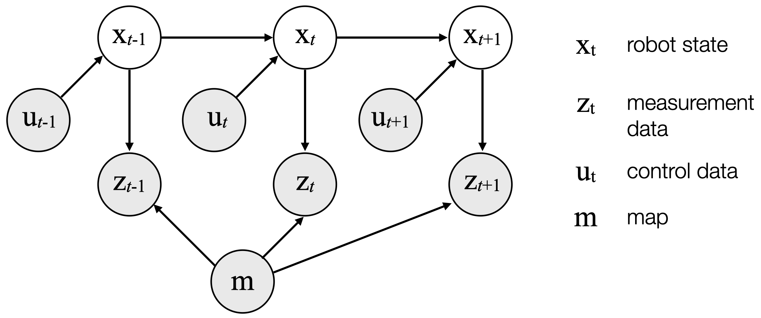
Today, we're building upon the robot state estimation concepts we covered in our last class meeting the by formulating the problem of robot localization as a state estimation problem. For robot localization, $x_t$ represents the location and orientation of the robot, $u_t$ represents the movements of the robot, and $z_t$ represents the sensor measurements available to the robot (typically a LiDAR or another sensor that measures the distance from the robot to its surroundings).

Robot localization seeks to answer the question of "where am I?" from the robot's perspective. One important assumption of robot localization is that the robot has access to a map of the environment. This map will inform the measurement update in the filtering algorithm we'll use to update the robot's belief of where it is in the world relative to the map.

Monte Carlo Localization (MCL) Algorithm

$\textrm{Algorithm MCL}( \mathcal{X}_{t-1}, u_t, z_t, \mathcal{M}):$
$\qquad \overline{\mathcal{X}_{t}} = \mathcal{X}_{t} = \emptyset $
$\qquad \textrm{for} \: m = 1 \: \textrm{to} \: M \: \textrm{do} $
$\qquad \qquad x_t^{[m]} = \textrm{sample_motion_model}(u_t, x_{t-1}^{[m]}) $
$\qquad \qquad w_t^{[m]} = \textrm{measurement_model}(z_t, x_{t}^{[m]}, \mathcal{M}) $
$\qquad \qquad \overline{\mathcal{X}_{t}} = \overline{\mathcal{X}_{t}} + \langle x_t^{[m]} , w_t^{[m]} \rangle $
$\qquad \textrm{end for} $
$\qquad \textrm{for} \: m = 1 \: \textrm{to} \: M \: \textrm{do} $
$\qquad \qquad \textrm{draw} \: i \: \textrm{with} \: \textrm{probability} \propto w_t^{[i]}$
$\qquad \qquad \textrm{add} \: x_t^{[i]} \: \textrm{to} \: \mathcal{X}_{t}$
$\qquad \textrm{end for} $
$\qquad \textrm{return} \: \mathcal{X}_{t} $

Here, we detail what each of the variables and symbols represent in the MCL algorithm above:

$\mathcal{X}_{t}$ is a set of $M$ particles representing the belief $bel(x_t)$, where the $m$-th particle in $\mathcal{X}_{t}$ is represented as $x_t^{[m]}$
$u_t$ represents the actions of the robot (i.e., control data) at time $t$
$z_t$ represents the measurement data the robot receives (i.e., sensor data) at time $t$
$\mathcal{M}$ represents the map the robot has access to of its environment
$\mathcal{W}_{t}$ is a set of $M$ particles representing the particle importance weights, where the $m$-th particle in $\mathcal{W}_{t}$ is represented as $w_t^{[m]}$
$\propto$ is equivalent to "proportional to"

Class Exercise: Monte Carlo Localization on Paper

For this exercise, use scratch paper or an electronic equivalent - DO NOT complete this exercise using code. In prior classes where students completed this exercise, many of them found that screen sharing and annotating the screen on Zoom was helpful to keep track of the particle movements.

Move, Compute Weights, Resample

Let's start out by imagining that our robot is in a 2D grid world (pictured below).

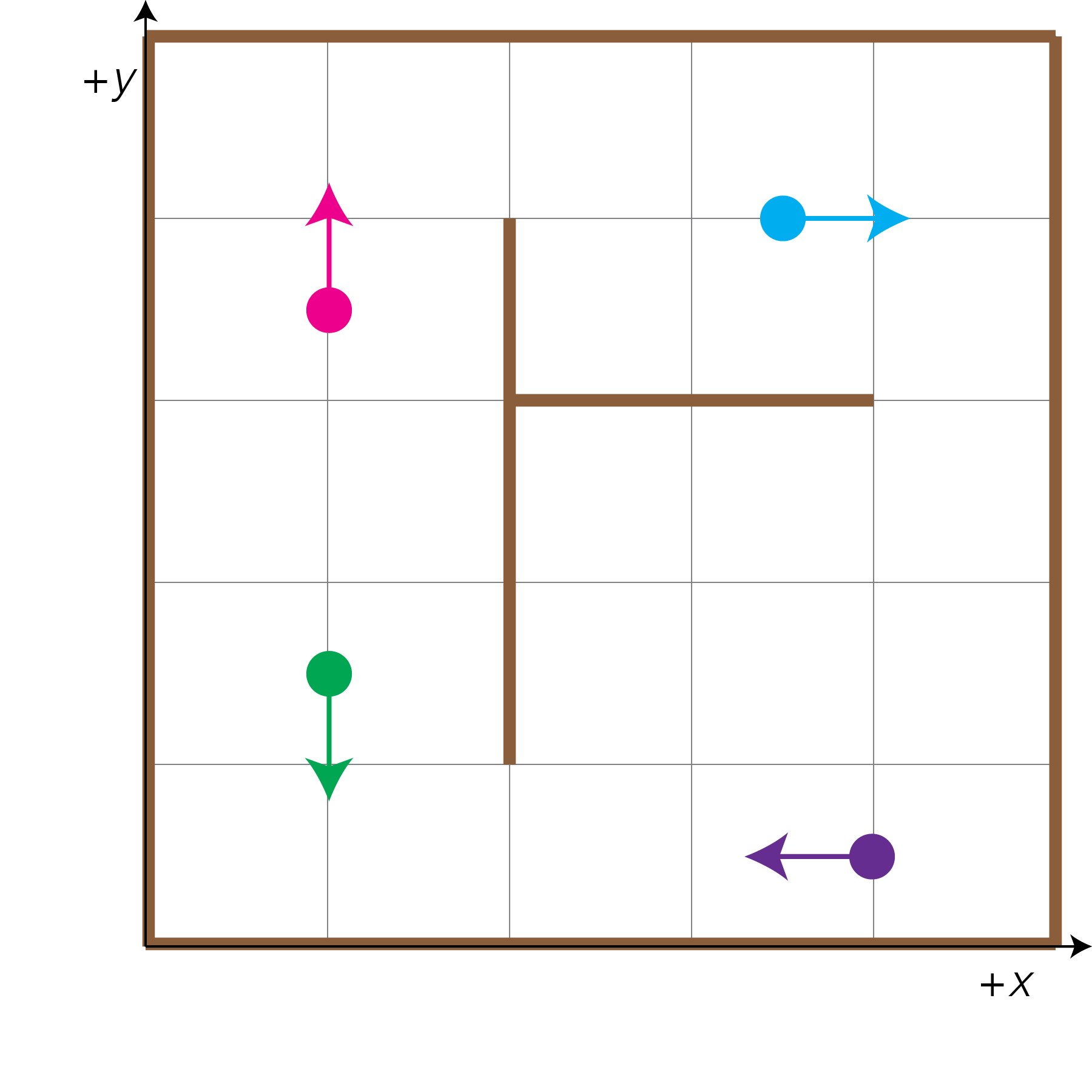
We have 4 guesses of where we think our robot is in the world, represented by the following "particles" with locations in [x, y, Θ]:

The green particle at location [1.0, 1.5, 270°]
The pink particle at location [1.0, 3.5, 90°]
The blue particle at location [3.5, 4.0, 0°]
The purple particle at location [4.0, 0.5, 180°]

Additionally, it's important to know that our robot has 3 distance sensors:

1 sensor that tells the robot the distance to the closest obstacle to its left,
1 sensor that tells the robot the distance to the closest obstacle in front of it, and
1 sensor that tells the robot the distance to the closest obstacle to its right.

We will represent sensor measurement $z_t$ as an array of 3 values representing the left, front, and sensor measurements in that order. For example, if our robot were at the location and direction [1.0, 2.0, 90°], our robot's sensor readings would be $z_t = $ [1.0, 3.0, 1.0].

In order to determine which of these guesses corresponds with our robot's true location in the 2D world, we will iterate through the following process:

Move: Our robot will move in the environment. We must move our particles the same amount that the robot moved, computing their new [x, y, Θ] locations. For example, if our robot moves 1 unit forward, the purple particle will move from [4.0, 0.5, 180°] to [3.0, 0.5, 180°].

Compute Weights: Now, we must compare the robot's actual sensor readings with each particle's hypothetical sensor readings and assign a weight to each particle, where higher weight values indicates higher similarity with the robot's sensor readings.
- Our robot will receive readings from its 3 sensors. We must calculate the "sensor readings" each particle theoretically would make if the robot was actually in the particle's location ($z_t^{[m]} $). For example, if our robot were at the location and direction indicated by the purple particle, our robot's sensor readings would be [0.5, 4.0, 2.5].
- For this exercise, we will use the following measurement model to compute the importance weights for each particle ($m$): $$w_t^{[m]} = \frac{1}{\sum_{i = 0}^2 \textrm{abs}(z_t[i] - z_t^{[m]}[i])}$$

Resample: Proportional to the weights you just computed for each of the particles, sample with replacement (resample), a new set of particles.
- First, you'll need to normalize your particle importance weights such that $\sum_m w_t^{[m]} = 1 $.
- Then, you'll need to sample with replacement a new set of 4 particles with probability proportional to the importance weights $w_t^{[m]}$. For the purposes of this class exercise, please pretend one of you is a random sampling algorithm and select 4 particles approximately proportional to their normalized importance weights. Please do not use code to do this, this exercise is intended to be completed with pen and paper.

For each of the following time steps (with its corresponding robot movements and sensor readings), go through the three steps above to execute this simplified version of a particle filter to localize the robot:

$t = 1$
- Robot movement ($u_t$): move forward 1.0 unit
- Robot sensor readings ($z_t$): [1.5, 0.5, 3.5]
$t = 2$
- Robot movement ($u_t$): turn 90° clockwise
- Robot sensor readings ($z_t$): [0.5, 3.5, 4.5]
$t = 3$
- Robot movement ($u_t$): move forward 1.5 units
- Robot sensor readings ($z_t$): [0.5, 2.0, 1.5]

Once you finish calculating going through the move, compute weights, and resample steps for each of the three timesteps you can check your solutions on this Monte Carlo localization exercise solutions page.

Acknowledgments

This page and the content for today's lecture were informed by Probabilistic Robotics by Sebastian Thrun, Wolfram Burgard, and Dieter Fox. The idea class exercise for today was developed in collaboration with Keely Haverstock.