Class Meeting 04: Monte Carlo Localization Exercise Solutions

This page contains solutions for the Monte Carlo localization exercise in Class Meeting 04.

Start

To start, we have the following map of particles

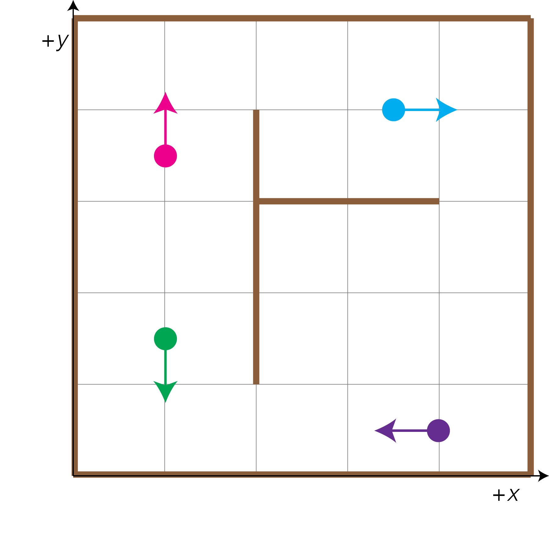
with the following locations:

The green particle at location [1.0, 1.5, 270°]
The pink particle at location [1.0, 3.5, 90°]
The blue particle at location [3.5, 4.0, 0°]
The purple particle at location [4.0, 0.5, 180°]

Additionally, our robot's sensors measurements \(z_t\) are represented as an array of 3 values representing the front, right and left sensor measurements.

\(t = 1\)

For \(t = 1\), our robot movement & sensor updates are:

Robot movement (\(u_t\)): move forward 1.0 unit
Robot sensor readings (\(z_t\)): [1.5, 0.5, 3.5]

Move: First, we must move each particle according to the robot's moment update. After moving forward each particle by 1.0, our map looks like

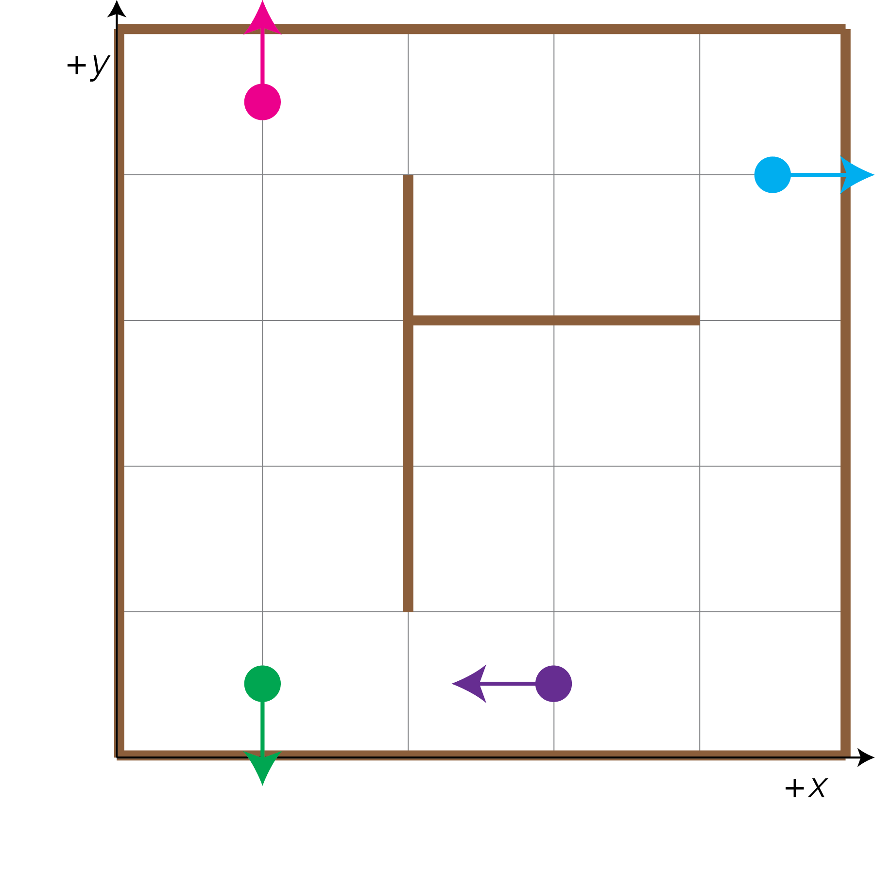
with the following locations and orientations of our particles:

The green particle at location [1.0, 0.5, 270°]
The pink particle at location [1.0, 4.5, 90°]
The blue particle at location [4.5, 4.0, 0°]
The purple particle at location [3.0, 0.5, 180°]

Compute Weights: To compute the particle weights, we must first calculate what the sensor measurements of the robot would be if it were in the position of each particle:

The green particle would have sensor measurements of \(z_1^{[green]} = [4.0, 0.5, 1.0]\)
The pink particle would have sensor measurements of \( z_1^{[pink]} = [1.0, 0.5, 4.0]\)
The blue particle would have sensor measurements of \(z_1^{[blue]} = [1.0, 0.5, 4.0]\)
The purple particle would have sensor measurements of \(z_1^{[purple]} = [0.5, 3.0, 2.5]\)

Next, we compute the weights for each particle for \(t=1\):

\(w_1^{[green]}\) \(= \frac{1}{\sum_{i = 0}^2 \textrm{abs}(z_1[i] - z_1^{[green]}[i])} = \frac{1}{\textrm{abs}(1.5 - 4.0) + \textrm{abs}(0.5 - 0.5) + \textrm{abs}(3.5 -1.0)} = \frac{1}{2.5 + 0 + 2.5} = \frac{1}{5} = 0.20\)
\(w_1^{[pink]}\) \(= \frac{1}{\sum_{i = 0}^2 \textrm{abs}(z_1[i] - z_1^{[pink]}[i])} = \frac{1}{\textrm{abs}(1.5 - 1.0) + \textrm{abs}(0.5 - 0.5) + \textrm{abs}(3.5 - 4.0)} = \frac{1}{0.5 + 0 + 0.5} = \frac{1}{1} = 1.00\)
\(w_1^{[blue]}\) \(= \frac{1}{\sum_{i = 0}^2 \textrm{abs}(z_1[i] - z_1^{[blue]}[i])} = \frac{1}{\textrm{abs}(1.5 - 1.0) + \textrm{abs}(0.5 - 0.5) + \textrm{abs}(3.5 - 4.0)} = \frac{1}{0.5 + 0 + 0.5} = \frac{1}{1} = 1.00\)
\(w_1^{[purple]}\) \(= \frac{1}{\sum_{i = 0}^2 \textrm{abs}(z_1[i] - z_1^{[purple]}[i])} = \frac{1}{\textrm{abs}(1.5 - 0.5) + \textrm{abs}(0.5 - 3.0) + \textrm{abs}(3.5 - 2.5)} = \frac{1}{1 + 2.5 + 1} = \frac{1}{4.5} = 0.22\)

Resample: We'll first normalize the particle weights so that \(\sum_m w_1^{[m]} = 1 \). The current sum of the particles is \(2.42\).

\(w_1^{[green]}\) \(= \frac{0.20}{2.42} = 0.083\)
\(w_1^{[pink]}\) \(= \frac{1.00}{2.42} = 0.413\)
\(w_1^{[blue]}\) \(= \frac{1.00}{2.42} = 0.413\)
\(w_1^{[purple]}\) \(= \frac{0.22}{2.42} = 0.091\)

The selection of particles will be specific to your group. A likely result would be having 2 pink particles and 2 blue particles survive this resampling step. Another possible result would be having 1 particle that's either green or purple and 3 particles that are either pink or blue. For the purposes of the solutions, we will assume that you choose 1 of each color particle, so that we have a full solution set. However, it is expected that you will not keep each color particle around for each iteration of the algorithm.

\(t = 2\)

For \(t = 2\), our robot movement & sensor updates are:

Robot movement (\(u_t\)): turn 90° clockwise
Robot sensor readings (\(z_t\)): [0.5, 3.5, 4.5]

Move: Again, our first step is to move each particle according to the robot's moment update. After rotating each particle clockwise by 90°, our map looks like

with the following locations and orientations of our particles:

The green particle at location [1.0, 0.5, 180°]
The pink particle at location [1.0, 4.5, 0°]
The blue particle at location [4.5, 4.0, 270°]
The purple particle at location [3.0, 0.5, 90°]

Compute Weights: To compute the particle weights, we must first calculate what the sensor measurements of the robot would be if it were in the position of each particle:

The green particle would have sensor measurements of \(z_2^{[green]} = [0.5, 1.0, 4.5]\)
The pink particle would have sensor measurements of \( z_2^{[pink]} = [0.5, 4.0, 4.5]\)
The blue particle would have sensor measurements of \(z_2^{[blue]} = [0.5, 4.0, 2.5]\)
The purple particle would have sensor measurements of \(z_2^{[purple]} = [3.0, 2.5, 2.0]\)

Next, we compute the weights for each particle for \(t=2\):

\(w_2^{[green]}\) \(= \frac{1}{\sum_{i = 0}^2 \textrm{abs}(z_2[i] - z_2^{[green]}[i])} = \frac{1}{\textrm{abs}(0.5 - 0.5) + \textrm{abs}(3.5 - 1.0) + \textrm{abs}(4.5 -4.5)} = \frac{1}{0 + 2.5 + 0} = \frac{1}{2.5} = 0.40\)
\(w_2^{[pink]}\) \(= \frac{1}{\sum_{i = 0}^2 \textrm{abs}(z_2[i] - z_2^{[pink]}[i])} = \frac{1}{\textrm{abs}(0.5 - 0.5) + \textrm{abs}(3.5 - 4.0) + \textrm{abs}(4.5 - 4.5)} = \frac{1}{0 + 0.5 + 0} = \frac{1}{0.5} = 2.00\)
\(w_2^{[blue]}\) \(= \frac{1}{\sum_{i = 0}^2 \textrm{abs}(z_2[i] - z_2^{[blue]}[i])} = \frac{1}{\textrm{abs}(0.5 - 0.5) + \textrm{abs}(3.5 - 4.0) + \textrm{abs}(4.5 - 2.5)} = \frac{1}{0 + 0.5 + 2.0} = \frac{1}{2.5} = 0.40\)
\(w_2^{[purple]}\) \(= \frac{1}{\sum_{i = 0}^2 \textrm{abs}(z_2[i] - z_2^{[purple]}[i])} = \frac{1}{\textrm{abs}(0.5 - 3.0) + \textrm{abs}(3.5 - 2.5) + \textrm{abs}(4.5 - 2.0)} = \frac{1}{2.5 + 1.0 + 2.5} = \frac{1}{6} = 0.17\)

Resample: We'll first normalize the particle weights so that \(\sum_m w_2^{[m]} = 1 \). The current sum of the particles is \(2.97\).

Note: If you have a different particle set at this point, your resampling step will be different. Use this as a guide/example as opposed to the answer you should be getting. The same is true for the resample step for \(t = 3\).

\(w_1^{[green]}\) \(= \frac{0.40}{2.97} = 0.135\)
\(w_1^{[pink]}\) \(= \frac{2.00}{2.97} = 0.673\)
\(w_1^{[blue]}\) \(= \frac{0.4}{2.97} = 0.135\)
\(w_1^{[purple]}\) \(= \frac{0.17}{2.97} = 0.057\)

\(t = 3\)

For \(t = 3\), our robot movement & sensor updates are:

Robot movement (\(u_t\)): move forward 1.5 units
Robot sensor readings (\(z_t\)): [0.5, 2.0, 1.5]

Move: For our \(t = 3\) movement update, we must again move each particle according to the robot's moment update. After moving forward each particle by 1.5, our map looks like

with the following locations and orientations of our particles:

The green particle at location [-0.5, 0.5, 180°]
The pink particle at location [2.5, 4.5, 0°]
The blue particle at location [4.5, 2.5, 270°]
The purple particle at location [3.0, 2.0, 90°]

Compute Weights: To compute the particle weights, we must first calculate what the sensor measurements of the robot would be if it were in the position of each particle:

The green particle would have sensor measurements of \(z_3^{[green]} = [\infty, \infty, \infty]\)
The pink particle would have sensor measurements of \( z_3^{[pink]} = [0.5, 2.5, 1.5]\)
The blue particle would have sensor measurements of \(z_3^{[blue]} = [0.5, 2.5, 2.5]\)
The purple particle would have sensor measurements of \(z_3^{[purple]} = [1.0, 1.0, 2.0]\)

Next, we compute the weights for each particle for \(t=3\):

\(w_3^{[green]}\) \(= \frac{1}{\sum_{i = 0}^2 \textrm{abs}(z_3[i] - z_3^{[green]}[i])} = \frac{1}{\textrm{abs}(0.5 - \infty) + \textrm{abs}(2.0 - \infty) + \textrm{abs}(1.5 - \infty)} = \frac{1}{\infty + \infty + \infty} = \frac{1}{\infty} = 0.00\)
\(w_3^{[pink]}\) \(= \frac{1}{\sum_{i = 0}^2 \textrm{abs}(z_3[i] - z_3^{[pink]}[i])} = \frac{1}{\textrm{abs}(0.5 - 0.5) + \textrm{abs}(2.0 - 2.5) + \textrm{abs}(1.5 - 1.5)} = \frac{1}{0 + 0.5 + 0} = \frac{1}{0.5} = 2.00\)
\(w_3^{[blue]}\) \(= \frac{1}{\sum_{i = 0}^2 \textrm{abs}(z_3[i] - z_3^{[blue]}[i])} = \frac{1}{\textrm{abs}(0.5 - 0.5) + \textrm{abs}(2.0 - 2.5) + \textrm{abs}(1.5 - 2.5)} = \frac{1}{0 + 0.5 + 1.0} = \frac{1}{1.5} = 0.67\)
\(w_3^{[purple]}\) \(= \frac{1}{\sum_{i = 0}^2 \textrm{abs}(z_3[i] - z_3^{[purple]}[i])} = \frac{1}{\textrm{abs}(0.5 - 1.0) + \textrm{abs}(2.0 - 1.0) + \textrm{abs}(1.5 - 2.0)} = \frac{1}{0.5 + 1.0 + 0.5} = \frac{1}{2} = 0.50\)

Resample: We'll first normalize the particle weights so that \(\sum_m w_3^{[m]} = 1 \). The current sum of the particles is \(3.17\).

\(w_1^{[green]}\) \(= \frac{0.00}{3.17} = 0.000\)
\(w_1^{[pink]}\) \(= \frac{2.00}{3.17} = 0.631\)
\(w_1^{[blue]}\) \(= \frac{0.67}{3.17} = 0.211\)
\(w_1^{[purple]}\) \(= \frac{0.50}{3.17} = 0.158\)

End of the exercise

At this point, it should be clear that the pink particle, out of the four, is the best guess to the true location of the robot. If you were wondering, the robot was actually located originally at [1.5, 3.5, 90°].