Class Meeting 05: Measurement Models for Range Finders and SLAM

Today's Class Meeting

Learning about two measurement models for range finders (Beam Models and Likelihood Fields) - here's a link to today's slides
Implementing the likelihood field for range finders algorithm with pen & paper
Covering a brief overview of Simultaneous Localization and Mapping (SLAM) as a primer for our next lab

What You'll Need for Today's Class

For today's class, you'll need the following tools/applications ready and running:

Your Ubuntu 20.04 programming environment
Your particle filter localization project partner

Beam Models of Range Finders

Here, we detail a beam model for range finders algorithm.

$\textrm{Algorithm beam_range_finder_model}(z_t, x_t, m):$
$ \qquad q = 1 $
$ \qquad \textrm{for} \: k = 1 \: \textrm{to} \: K \: \textrm{do} $
$ \qquad\qquad \textrm{compute} \: z_t^{k*} \: \textrm{for the measurement} \: z_t^{k} \: \textrm{using ray casting} $
$ \qquad\qquad p = z_{hit} \cdot p_{hit}(z_t^k|x_t,m) + z_{short} \cdot p_{short}(z_t^k|x_t,m) + z_{max} \cdot p_{max}(z_t^k|x_t,m) + z_{rand} \cdot p_{rand}(z_t^k|x_t,m) $
$ \qquad\qquad q = q \cdot p$
$ \qquad \textrm{return} \: q $

Here, we provide additional details on the algorithm above:

$ z_t $ represents the laser range finder measurements received by the robot where $ z_t^k $ represents the $ k$-th range finder measurement
$ z_t^{k*}$ represents the "true" sensor measurement the robot would have read if it had been in the location we believe it to be in (i.e., the particle sensor measurement)
$ x_t $ represents the location we believe we are in (i.e., the particle location)
$ m $ represents the map of the world
the algorithm line $ q = q \cdot p $ comes from the way we incorporate all of the $K$ readings from the laser range finder, $p(z_t|x_t,m) = \prod_{k=1}^K p(z_t^k|x_t,m)$
$ (z_{hit} + z_{short} + z_{max} + z_{rand}) = 1 $

Accounting for possible measurement error in beam models

The beam model of range finders accounts for 4 types of possible measurement error: measurement noise, unexpected objects, failure to detect obstacles, and random measurements.

Measurement noise is accounted for through $ p_{hit}(z_t^k | x_t, m) $ according to: $$p_{hit}(z_t^k | x_t, m) = \{ \: \eta \mathcal{N}(z_t^k;z_t^{k*},\sigma_{hit}^2), \:\: \textrm{if} \: 0 \le z_t^k \le z_{max} \: ; \: 0, \: \textrm{otherwise} \}$$ where $\mathcal{N}(z_t^k;z_t^k*,\sigma_{hit}^2)$ denotes the univariate normal distribution with mean $z_t^{k*}$ and standard deviation $\sigma_{hit}$, and $\eta$ is a normalizing constant.

Unexpected objects (e.g., a person walking through the space that isn't captured in our static map) is accounted for through $ p_{short}(z_t^k | x_t, m)$ according to: $$p_{short}(z_t^k | x_t, m) = \{ \: \eta \lambda_{short} e^{-\lambda_{short}z_t^k}, \:\: \textrm{if} \: 0 \le z_t^k \le z_t^{k*} \: ; \: 0, \: \textrm{otherwise} \} $$ where $\lambda_{short}$ is an intrinsic parameter of the measurement model, and $\eta$ is a normalizing constant.

We account for a possible failure to detect obstacles assuming that failures result in a max-range measurement (due to, for example, sensing black light-absorbing objects or measuring objects in bright sunlights) according to: $$p_{max}(z_t^k | x_t, m) = \{ \: 1 \: \textrm{if} \: z = z_{max}, \: 0 \: \textrm{otherwise} \: \}$$

Finally, we account for random measurements according to: $$p_{rand}(z_t^k | x_t, m) = \{ \: \frac{1}{z_{max}} \textrm{if} \: 0 \le z_t^k \le z_{max}, \: 0 \: \textrm{otherwise} \: \}$$

Likelihood Fields for Range Finders

Here, we detail a likelihood field for range finders algorithm.

$ \textrm{Algorithm likelihood_field_range_finder_model}(z_t, x_t, m): $
$ \qquad q = 1 $
$ \qquad \textrm{for} \: k = 1 \: \textrm{to} \: K \: \textrm{do} $
$ \qquad \qquad \textrm{if} \: z_t^k \ne z_{max} $
$ \qquad \qquad \qquad x_{z_t^k} = x + x_{k,sens} cos \theta - y_{k,sens} sin \theta + z_t^k cos \big( \theta + \theta_{k,sens} \big) $
$ \qquad \qquad \qquad y_{z_t^k} = y + y_{k,sens} cos \theta - x_{k,sens} sin \theta + z_t^k sin \big( \theta + \theta_{k,sens} \big) $
$ \qquad \qquad \qquad dist = \textrm{min}_{x', y'} \: \Big\{ \sqrt{(x_{z_t^k} - x')^2 + (y_{z_t^k} - y')^2} \Big| \langle x', y' \rangle \: \textrm{occupied in } m \Big\} $
$ \qquad \qquad \qquad q = q \cdot \bigg( z_{hit} \: \textrm{prob}(dist,\sigma_{hit}) + \frac{z_{random}}{z_{max}} \bigg) $
$ \qquad \textrm{return} \: q $

Here, we provide additional details on the algorithm above:

$ z_t $ represents the laser range finder measurements received by the robot where $ z_t^k $ represents the $ k$-th range finder measurement and $ z_{max} $ represents the maximum possible value of the range finder
$ x_t = (x, y, \theta)^T$ represents the location we believe we are in (i.e., the particle location)
$ m $ represents the map of the world
$x_{k,sens}$, $y_{k,sens}$, and $\theta_{k,sens}$ represent the the location and orientation of the robot's sensor relative to the robot's position and heading (for our Turtlebot3, we can make the assumption that $x_{k,sens} = 0$ and $y_{k,sens} = 0$ ). $\theta_{k,sens}$ will be equal to the angle at which the LiDAR is taking the sensor reading.
$\textrm{prob}(dist,\sigma_{hit}) $ is a zero-centered Gaussian with a standard deviation of $\sigma_{hit}$, where a zero-centered Gaussian distribution can be represented as $ g(x) = \frac{1}{\sigma{ \sqrt (2 \pi)}} e^{-x^2/2 \sigma^2} $
the algorithm line $ q = q \cdot \bigg( z_{hit} \: \textrm{prob}(dist,\sigma_{hit}) + \frac{z_{random}}{z_{max}} \bigg) $ comes from the way we incorporate all of the $K$ readings from the laser range finder, $p(z_t|x_t,m) = \prod_{k=1}^K p(z_t^k|x_t,m)$
$ (z_{hit} + z_{max} + z_{rand}) = 1 $

Note: For your particle filter project, you don't need to necessarily "skip" $ z_{max} $ values as this $ \textrm{likelihood_field_range_finder_model}$ algorithm specifies. What you want to do is think carefully about the scenarios where you may encounter $ z_{max} $ values, and then multiply $ q $ by a value that makes sense.

Class Exercise: Using a Likelihood Field Approach for a Measurement Model for Monte Carlo Localization

We are going to repeat the exercise from Class Meeting 04, but instead of completing the measurement model using a ray casting approach, we'll use a likelihood field approach.

Exercise Setup

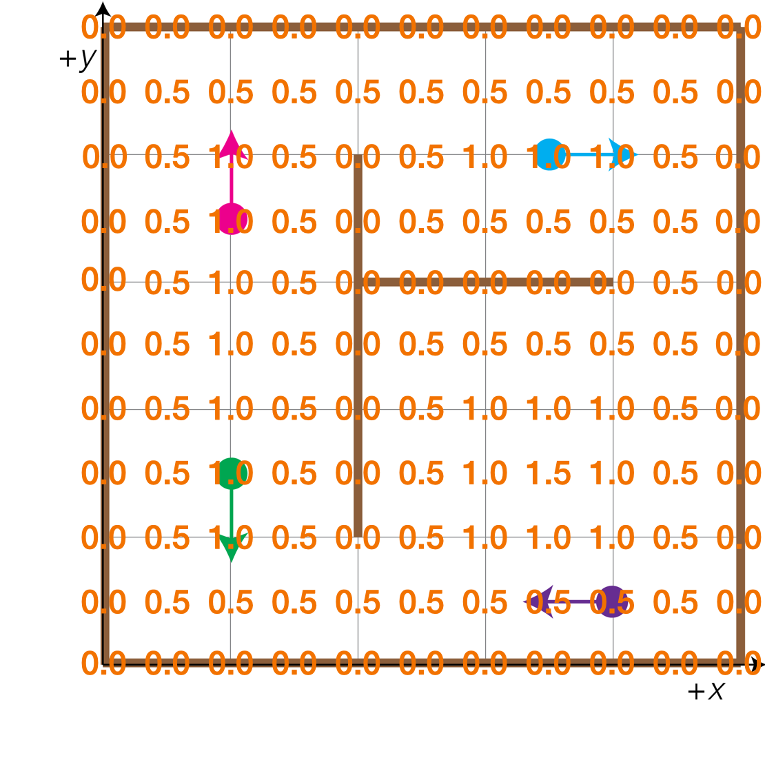
We'll use the same 2D grid world that we did before (pictured below on the left) as well as the likelihood field for this grid world (pictured below on the right).

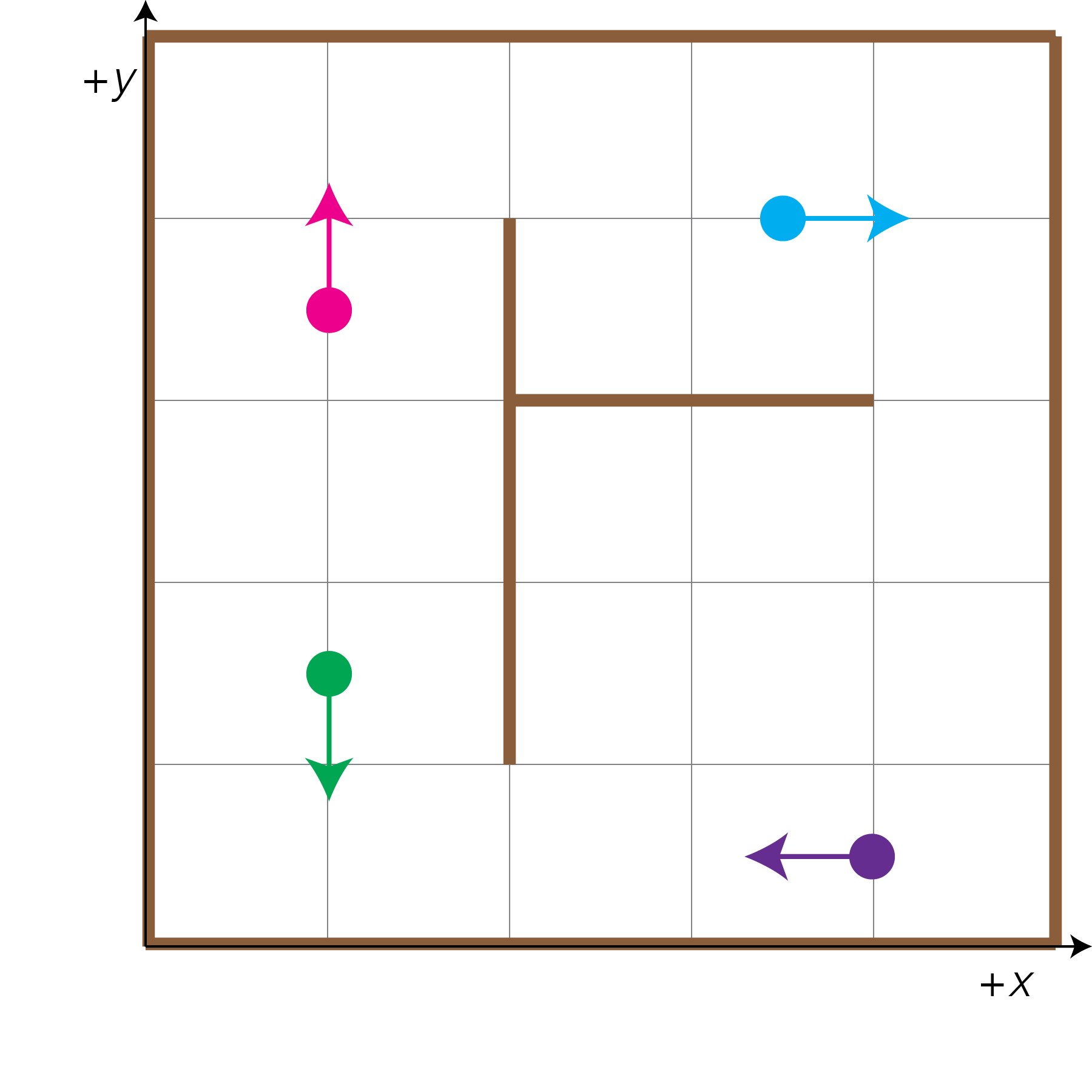
Again, our particles are located at the following positions represented as [x, y, Θ]:

The green particle at location [1.0, 1.5, 270°]
The pink particle at location [1.0, 3.5, 90°]
The blue particle at location [3.5, 4.0, 0°]
The purple particle at location [4.0, 0.5, 180°]

We represent sensor measurement $z_t$ as an array of 3 values representing the left, front, and sensor measurements in that order. For example, if our robot were at the location and direction [1.0, 2.0, 90°], our robot's sensor readings would be $z_t = $ [1.0, 3.0, 1.0].

In order to determine which of these guesses corresponds with our robot's true location in the 2D world, we will again iterate through the following process:

Move: Our robot will move in the environment. We must move our particles the same amount that the robot moved, computing their new [x, y, Θ] locations.

Compute Weights: This is the component that is unique and distinct from last class, since we'll be using a likelihood field approach for the measurement model instead of ray casting. This will allow us to compute particle weights, where high weights values indicate higher similarity with the robot's sensor readings.
- Our robot will receive readings from its 3 sensors. Using these sensor readings and the likelihood field provided above, you'll need to compute $dist_{closest\_obs}$, the distance to the closest obstacle based on the likelihood field algorithm, for each robot sensor reading.
- For this exercise, we will use the following measurement model to compute the importance weights for each particle ($m$): $$w_t^{[m]} = \frac{1}{\sum_{i = 0}^2 dist_{closest\_obs}[i]}$$

Resample: Proportional to the weights you just computed for each of the particles, sample with replacement (resample), a new set of particles.
- First, you'll need to normalize your particle importance weights such that $\sum_m w_t^{[m]} = 1 $.
- Then, you'll need to sample with replacement a new set of 4 particles with probability proportional to the importance weights $w_t^{[m]}$. For the purposes of this class exercise, please pretend one of you is a random sampling algorithm and select 4 particles approximately proportional to their normalized importance weights. Please do not use code to do this, this exercise is intended to be completed with pen and paper.

For each of the following time steps (with its corresponding robot movements and sensor readings), go through the three steps above to execute this simplified version of a particle filter to localize the robot:

$t = 1$
- Robot movement ($u_t$): move forward 1.0 unit
- Robot sensor readings ($z_t$): [1.5, 0.5, 3.5]
$t = 2$
- Robot movement ($u_t$): turn 90° clockwise
- Robot sensor readings ($z_t$): [0.5, 3.5, 4.5]
$t = 3$
- Robot movement ($u_t$): move forward 1.5 units
- Robot sensor readings ($z_t$): [0.5, 2.0, 1.5]

Once you finish calculating going through the move, compute weights, and resample steps for each of the three timesteps you can check your solutions on this Likelihood Field exercise solutions page.

Acknowledgments

This page and the content for today's lecture were informed by Probabilistic Robotics by Sebastian Thrun, Wolfram Burgard, and Dieter Fox.